4 Session 4: Biological tables, plots and linear models in R
4.1 Overview
ImportantClearer wording of the workbook questions (click to open)
Some workbook questions were not worded clearly enough. Below, each one is shown as it is in your workbook (before), then reworded (after). They ask exactly the same thing: keep answering in your own WORKBOOK.qmd, under the same question number.
A1
Before: How many rows and columns does plants have? What does one row represent? Many biomass values are NA: what does that mean?
After:
- How many rows and how many columns does the table
plantshave? - What does one row of the table describe?
- Many values in the biomass columns are
NA. What doesNAmean here?
B1
Before: How many plants had each job? Which job gave the bacteria of the rhizoplane, and which one gave the bacteria of the bulk soil? (See the table in the theory part.)
After:
Look at the column analysis: it says what each plant was used for.
- How many plants were used for each type of analysis?
- The rhizoplane bacteria were sampled on the plants of one type of analysis, and the bulk soil bacteria on the plants of another. Which ones? (Help: the table “each plant had one job” in the theory part of the session page.)
B2
Before: Are the watered and drought rhizotubes grouped or mixed? Why would an experimenter mix them on purpose? What do you notice when you compare the two maps?
After:
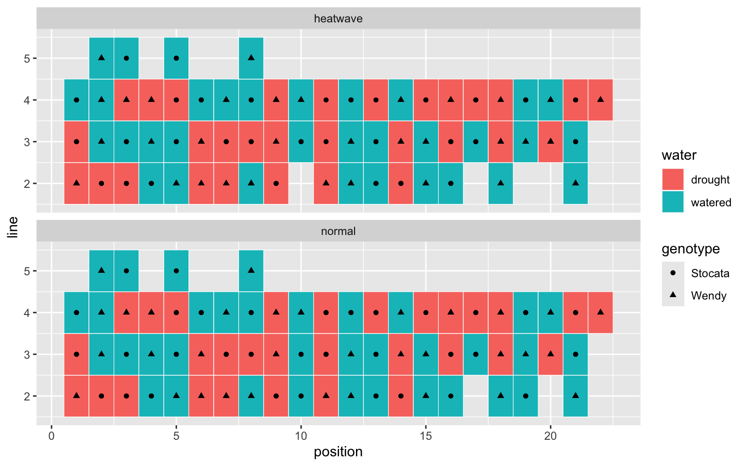
On the map, each coloured square is one rhizotube.
- Are the drought rhizotubes all together in one area, or mixed with the watered ones?
- Why would a scientist mix them on purpose?
- Compare the two maps (heatwave and normal). What do you notice?
B4
Before: How many plants were weighed? Copy the four mean biomasses (2 decimals). Which stress weighs more on the plant, drought or the heatwave?
After:
- How many plants were weighed?
- Copy the four mean biomasses (2 decimals).
- Which stress reduces the biomass of the plant more: drought or the heatwave?
B5
Before: How many rows does organs have, and why exactly that number? Under drought, which organ keeps the largest share of its biomass (to be sure, compute the mean per organ and water regime, as in B4), and why could that help a plant that is short of water?
After:
- How many rows does the table
organshave? Why exactly this number? - Under drought, which organ (leaf, stem or root) loses the smallest percentage of its biomass? To be sure, compute the mean biomass per organ and water regime, as in B4.
- Why could keeping its roots help a plant that does not have enough water?
C1
Before: Which compartments have fewer than 40 samples, and how many samples are missing in total?
After:
- Which compartments have fewer than 40 samples?
- How many samples are missing in total?
C2
Before: Which compartment has the most diverse bacteria, and which the least? According to the Tukey test, which pairs of compartments do not differ? Why could the bacteria inside the root be much less diverse than in the soil around it?
After:
- Which compartment has the most diverse bacteria, and which one the least diverse?
- In the Tukey table, which pairs of compartments are not significantly different (
p adjabove 0.05)? - Why could the bacteria inside the root be much less diverse than in the soil around it?
C3
Before: How many rhizoplane samples are there, and how many per combination?
After:
- How many rhizoplane samples are there?
- How many samples are there in each combination of water, heat and genotype?
C4
Before: Before any statistics: which factor (water, heat or genotype) seems to change Shannon diversity the most? Is it the same factor that weighed most on the plant’s biomass (B4)?
After:
Look at the plot only, before any statistics.
- Which factor seems to change the Shannon diversity the most: water, heat or genotype?
- Is it the same factor that reduced the biomass of the plants the most (B4)?
D1
Before: Mean Shannon diversity (2 decimals) of watered and of drought plants, and the t-test p-value:
After:
- Copy the mean Shannon diversity (2 decimals) of the watered plants and of the drought plants.
- Copy the p-value of the t-test.
D2
Before: What is the estimate of waterwatered, and how does it relate to your two means in D1? Compare its p.value with the t-test’s.
After:
In the table, find the row called waterwatered (the column water, level watered).
- What is its
estimate? - Compute the difference between your two means in D1. What do you notice?
- Is its
p.valuethe same as the p-value of the t-test?
D3
Before: Which rows of the ANOVA table have a p-value (Pr(>F)) below 0.05? Copy the p-value of water.
After:
- Which rows of the ANOVA table have a p-value (column
Pr(>F)) below 0.05? - Copy the p-value of
water.
D4
Before: What share of the variation (in %) does water explain? And the residuals? Was your guess in C4 right?
After:
- What percentage of the variation does
waterexplain? And theResiduals? - Was your guess in C4 correct?
D5
Before: What does the subtitle of your plot say, exactly? Why is it better to compute it in R than to type the number by hand?
After:
- Copy the subtitle of your plot, exactly.
- Why is it better to compute this p-value with R than to type the number by hand?
E1
Before: How many bulk soil samples are there, and how many per combination?
After:
- How many bulk soil samples are there?
- How many samples are there in each combination of water, heat and genotype?
E2
Before: Looking only at the plot: which factor moves the means the most, water or heat? Are the two lines roughly parallel, and what would it mean if they were not?
After:
Look at the plot only.
- Which factor changes the mean diversity the most: water (compare left and right on the x axis) or heat (compare the two lines)?
- Are the two lines more or less parallel?
- What would it mean if they were not parallel?
E3
Before: Which factor(s) have a p-value below 0.05 in the bulk soil, and what share of the variation does each explain? Using bulk_soil_means, how large is the heatwave effect in Shannon units? Compare it with the drought effect on the rhizoplane (D1).
After:
- Which factor(s) have a p-value below 0.05 in the bulk soil?
- What percentage of the variation does each of them explain?
- In
bulk_soil_means, by how much does the heatwave lower the mean Shannon diversity (normal minus heatwave)? Compare with the effect of drought on the rhizoplane (D1).
E5 (graded)
Before: Answer today’s biological question for the bulk soil, and compare it with the rhizoplane (4-6 sentences). Cite at least one mean, one p-value and one share of variation from your own results. Which factor matters in each compartment, and how much? By what mechanism could drought change the bacteria on the root surface, but not in the soil further from the root? Is the significant effect in the bulk soil also a large one? Refer to your figure with @fig-bulk.
After:
Answer today’s biological question for the bulk soil, and compare it with the rhizoplane, in 4-6 sentences. Your answer should:
- say which factor matters in the bulk soil and which one on the rhizoplane, and how much, with at least one mean, one p-value and one percentage of variation from your own results;
- explain how drought could change the bacteria on the root surface, but not in the soil further from the root (think of what the root releases and takes up);
- say whether the significant effect in the bulk soil is also a large one;
- refer to your figure with
@fig-bulk.
E6 (graded)
Before: One limitation, uncertainty or assumption of today’s analysis (think, for example, of the number of plants per group, of what the Shannon index does not tell you, or of the y axis of your plot):
After:
Give one limitation of today’s analysis: something that makes the conclusion less certain. Ideas: the number of plants per group, what the Shannon index does not tell you, or the y axis of your plot.
Download the lecture slides (PDF)
TipQuick poll (Poll Everywhere)
Respond at pe.app/cmaslard3
NoteBiological question
Soybean plants were grown under drought, a heatwave, or both. How much do these stresses hurt the plants, and do they also change how diverse the bacteria living on and around their roots are?
Sessions 1-3 were about sequences: reading them, checking them, comparing them. From today, the course moves to tables: one row per sample, one column per measurement. This is the kind of data you will meet in almost every biology project, whatever the organism or the technique.
Today’s tables are real data from the lab: a soybean experiment where two cultivars grew under four climates. You will start very gently, with a clean R project and the plants themselves: where they stood in the experiment, what each one was used for, and how much the stresses weighed on them. You will then turn to the bacteria living on and around them (16S amplicon sequencing), reshape and summarise the tables with dplyr and tidyr, draw clearer plots with ggplot2, run your first statistical tests, from a t-test to a linear model that says which part of the climate actually matters, and write their results on your plots.
ImportantHow you work and submit today
Everything happens in one file, WORKBOOK.qmd: your code, your plots and your answers together. When you click Render, it becomes one HTML page, and that page is what you submit. You start the workbook in class and submit it on Moodle by Sunday evening (18 October).
4.1.1 Learning outcomes
By the end of this session, you should be able to:
- organise an analysis as a clean R project (
data/,results/, one.qmdreport) and render it; - describe a table in terms of observations (rows) and variables (columns), and spot missing values and missing samples;
- explain the design of the soybean experiment, and why its plants were mixed in space;
- use five dplyr/tidyr verbs (
filter,mutate,group_by+summarise,count,pivot_longer) to prepare a table for a plot; - build a ggplot layer by layer: data, aesthetics, geometry, facets, including a map with
geom_tile(); - choose a test from a simple table (t-test, ANOVA, Tukey, linear model, and their alternatives);
- run a t-test, and explain why it is the same thing as a linear model with one factor;
- fit a linear model with several factors, read its ANOVA table, and say how much of the variation each factor explains;
- draw an interaction plot (means and error bars) and write a p-value on a plot;
- insert a saved figure into a Quarto report, with a caption and a cross-reference;
- tell apart a significant effect and a large effect.
4.1.2 Session plan
| Time | Block | What happens |
|---|---|---|
| 14:15-14:20 | Retrieval | Session 3 quiz, and who unknown_sample really was. |
| 14:20-14:35 | Theory 1 | A clean R project; tidy tables; the grammar of graphics. |
| 14:35-14:50 | Theory 2 | From a boxplot to a linear model; which test, when; the soybean experiment. |
| 14:50-15:00 | Practical briefing | What today’s workbook will ask of you. |
| 15:00-15:15 | Practical A | Build the R project, copy the data, render the workbook once. |
| 15:15-15:50 | Practical B | Meet the experiment: the plants, their map, their biomass. |
| 15:50-16:00 | Checkpoint | Map and biomass plots drawn. Short break. |
| 16:00-16:15 | Practical C | The bacteria: first look, then the rhizoplane. (pairs) |
| 16:15-16:35 | Practical D | Guided: the statistics, from a t-test to a linear model, and onto the plot. (pairs) |
| 16:35-16:55 | Practical E | Alone: an interaction plot and its statistics, for the bulk soil. |
| 16:55-17:00 | Wrap-up | Render, save, finish at home and submit by Sunday evening (18 October). |
4.2 Theory (≈45 min)
4.2.1 1. A clean R project
An analysis is not just a result: it is something another person (or you, in six months) must be able to rerun. The simplest habit that makes this possible is one folder per analysis, always organised the same way:
session_04/
├── session_04.Rproj      <- double-click to open the project in RStudio
├── WORKBOOK.qmd          <- your report: code + plots + text, in one file
├── data/                 <- raw data: read it, never edit it by hand
│   ├── soybean_plants.csv
│   └── soybean_alpha_diversity.csv
├── img/                  <- images you did not make with R (photos, schemes)
│   └── experimental_design.png
└── results/              <- everything your code produces (figures, tables)
Three rules come with it:
- Raw data is read-only. You never open the CSV in Excel to “fix” something: every change happens in code, so it is visible and repeatable.
- Paths are relative. Inside the project,
data/soybean_alpha_diversity.csvalways works, on any computer. A path likeC:/Users/me/Desktop/...only works on yours. - The report is the analysis. A Quarto file (
.qmd) mixes text and code chunks. When you Render it, R runs every chunk from top to bottom, in a clean session. If it renders, it is reproducible.
4.2.2 2. Tidy tables and the grammar of graphics
A tidy table has one row per observation (here: one sample) and one column per variable (compartment, water, heat, shannon, …). Almost every tool in R expects this shape.
The tidyverse is a family of packages built around tidy tables (each one is described in the R toolbox below). You will use three of them today:
- dplyr manipulates a table: keep some rows (
filter), add or change a column (mutate), summarise by group (group_by+summarise); - tidyr reshapes a table:
pivot_longerstacks several columns into one; - ggplot2 draws it. A ggplot is built in layers, joined with
+:
ggplot(data, aes(x = ..., y = ..., colour = ...)) +  # which table, which columns where
  geom_boxplot() +                                   # how to draw them
  facet_wrap(~ ...)                                  # one panel per group
Steps are chained with the pipe %>%, read as “and then”: take the table, and then keep the rhizoplane, and then compute the mean per group. It comes with the tidyverse, and RStudio types it for you with Ctrl/Cmd + Shift + M.
4.2.3 3. From a boxplot to a linear model
A boxplot shows that two groups look different. A statistical test answers whether that difference is larger than the noise between plants, and a linear model also says how large it is.
The key idea for this course: most common tests are the same linear model. A t-test comparing watered and drought plants is lm(shannon ~ water). Add a second factor and it becomes a two-way ANOVA: lm(shannon ~ water * heat). The * means “each factor, and their interaction”: does the effect of drought depend on the heatwave?
anova(model) then splits the total variation into one piece per factor, plus the residuals (what no factor explains: plant-to-plant noise). Two numbers matter for each factor:
- the p-value: could a difference this large appear by chance alone?
- the share of variation it explains (its sum of squares divided by the total): how much does it actually matter?
They are not the same thing. With very little noise, a tiny difference can be highly significant. Always look at both, and at the plot.
Which test, when? Keep this table at hand for the rest of the course. Each test assumes something about the data; when the assumption clearly fails, use the alternative in the last column.
| Your question | Example with today’s data | Test | In R | It assumes | If not |
|---|---|---|---|---|---|
| Do 2 groups differ? | Shannon, watered vs drought | Student’s t-test | t.test(y ~ group, var.equal = TRUE) |
values roughly normal, similar spread in both groups | Wilcoxon: wilcox.test(y ~ group) |
| Do 3 groups or more differ? (one factor) | Shannon across the 5 compartments | one-way ANOVA | anova(lm(y ~ group)) |
normal residuals, similar spread in all groups | Kruskal-Wallis: kruskal.test(y ~ group) |
| Which groups differ, after an ANOVA? | which compartments differ from which | Tukey HSD | TukeyHSD(aov(y ~ group)) |
same as the ANOVA | pairwise.wilcox.test(y, group, p.adjust.method = "BH") |
| Several factors at once, and their interactions? | water × heat × genotype | factorial ANOVA (a linear model) | anova(lm(y ~ a * b * c)) |
same as the ANOVA | transform y (for example log(y)) and refit |
| Are two measurements linked? | leaf biomass vs root biomass | correlation, or regression | cor.test(x, y), lm(y ~ x) |
a straight-line relationship | Spearman: cor.test(x, y, method = "spearman") |
How to check the assumptions of a model: look at its residuals with plot(model, which = 1) (spread) and plot(model, which = 2) (normality). Formal tests exist (shapiro.test(residuals(model))), but the plots tell you more.
4.2.4 4. Worked example: the soybean experiment
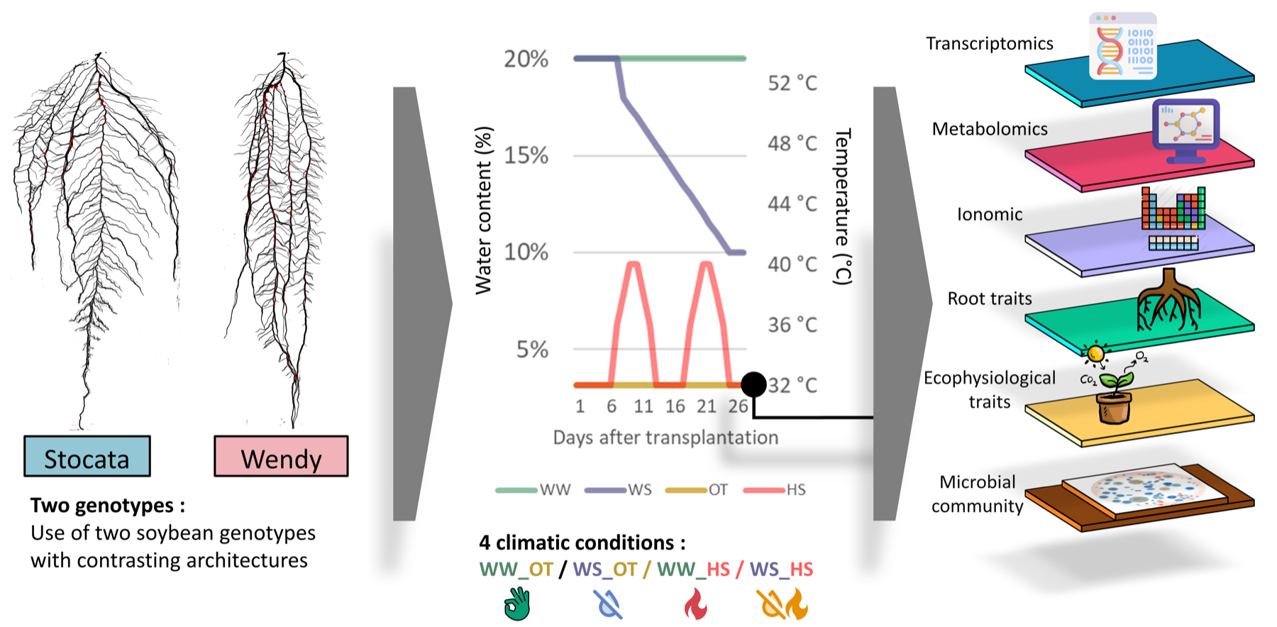
- 2 cultivars,
StocataandWendy, chosen for their contrasted root systems; - 4 climates: a factorial design of water (
watered, ordrought: watering slowly withdrawn from 20% to 10% soil water content) × temperature (normal, orheatwave: two waves at 40 °C for three days); - plants grew in rhizotubes: flat, transparent pots holding two plants of the same condition, set out in lines and positions (you will draw this map in block B);
- at the final harvest, each plant had one job, because most measurements destroy the plant:
analysis in your table |
What was done with this plant |
|---|---|
physiology |
dry biomass of each organ (leaf, stem, root), photosynthesis, water potential |
exudates |
molecules released by the roots, plus dry biomass |
omics_and_soil |
gene expression and metabolites of the organs; its soil gave the bulk soil and rhizosphere bacteria |
plant_microbiome |
the bacteria on and inside the plant: rhizoplane, root endosphere, phylloplane |
Two consequences you will meet today:
- the biomass and the bacteria were measured on different plants of the same conditions: you can compare conditions, but not link one plant’s biomass to its own bacteria;
- for the bacteria, each sample was sequenced (16S) and three alpha-diversity indices computed:
richness(how many different bacteria),evenness(how equally they share the space), andshannon(combines both; higher = more diverse).
4.2.5 Practical briefing
Today you work in pairs for blocks A-D, and alone for block E. Block B introduces the experiment through the plants: where they stood, what each one was used for, and how much the stresses weighed on them. Blocks C and D then turn to the bacteria and walk you through the full analysis on one compartment, the rhizoplane: a plot, then the statistics, then the statistics on the plot. In block E, you analyse the bulk soil on your own, with a different kind of figure: the reasoning is the same, the code and the answer are not. Your submission is the rendered workbook: your bulk soil figure, its statistics, and your interpretation are what is graded.
4.3 Your R toolbox
Read this once now, and come back to it whenever a function surprises you. One tab per package: what it is for, the functions you use today, one example, and the mistake everyone makes at least once.
What it is. Not one package but a family of packages designed to work together, all built around tidy tables. library(tidyverse) loads the core ones in one line, including the four below (readr, dplyr, tidyr, ggplot2) and the pipe %>%.
The pipe %>%. Passes what is on its left as the first argument of the function on its right. These two lines do exactly the same thing:
summarise(group_by(alpha, compartment), mean_shannon = mean(shannon))

alpha %>%
  group_by(compartment) %>%
  summarise(mean_shannon = mean(shannon))
The second one reads top to bottom, like a recipe. Shortcut in RStudio: Ctrl/Cmd + Shift + M.
Common mistake. Forgetting library(tidyverse) after restarting R: every tidyverse function then fails with could not find function. Rendering always starts from a fresh session, which is why library() lives in the first chunk of the workbook.
Go further. R for Data Science (free online book), and all the Posit cheat sheets.
What it is for. Reading rectangular text files (CSV, TSV) into R as a tibble, the tidyverse version of a table.
| Function | What it does |
|---|---|
read_csv("data/file.csv") |
read a comma-separated file |
read_tsv("data/file.tsv") |
read a tab-separated file |
write_csv(table, "results/file.csv") |
save a table you computed |
What to check. read_csv() guesses each column’s type and tells you what it found: chr (text) or dbl (number). Always glance at that message, or at glimpse(): a column of numbers read as chr means something in the file is not a number (a comma decimal, a “NA” typed as “n/a”, a unit in a cell…).
Common mistake. A path that only works on your computer ("C:/Users/me/Desktop/data.csv"). Inside an R project, always write the path from the project folder: "data/soybean_alpha_diversity.csv".
Cheat sheet. Data import with readr
What it is for. Manipulating a table: choosing rows, creating columns, summarising groups. Each function is a verb, takes a table first, and returns a new table.
| Verb | What it does | Today |
|---|---|---|
filter() |
keep the rows that match a condition | filter(compartment == "Rhizoplane") |
mutate() |
add a column or change one | mutate(compartment = factor(...)) |
count() |
count rows per group | count(alpha, compartment) |
group_by() + summarise() |
one summary row per group | group_by(water) %>% summarise(mean = mean(shannon)) |
is.na() |
TRUE where a value is missing; !is.na() keeps what is there |
filter(!is.na(biomass_total)) |
pull() |
take one column out of a table, as a plain value | filter(term == "heat") %>% pull(p.value) |
select(), arrange() |
keep some columns; sort rows | not needed today, good to know |
Example. Mean Shannon diversity per compartment and water regime, sorted:
alpha %>%
  group_by(compartment, water) %>%
  summarise(mean_shannon = mean(shannon)) %>%
  arrange(mean_shannon)
With two grouping columns, summarise() prints a message about “grouped output”: it is information, not an error.
Common mistakes.
=instead of==infilter().=gives a value to an argument,==tests equality. dplyr spots it and suggests the fix.- Forgetting the quotes:
filter(compartment == Rhizoplane)looks for a column calledRhizoplane. Values of text columns always go in quotes, column names never. - A
mutate()that is not saved:alpha %>% mutate(...)only shows the result. To keep it, assign it:alpha <- alpha %>% mutate(...).
Cheat sheet. Data transformation with dplyr
What it is for. Changing the shape of a table without changing its content.
- Wide: one row per plant, one column per measurement (
biomass_leaf,biomass_stem,biomass_root). Easy to read for a human, and the shape ofplants. - Long: one row per plant and organ, with a column saying which organ it is (
organ) and one with its value (biomass). The shape ggplot needs to put the organs side by side, or in their own panels.
| Function | What it does |
|---|---|
pivot_longer(cols, names_to, values_to) |
wide → long: stack several columns into two |
pivot_longer(..., names_prefix = "biomass_") |
the same, removing the start of the old column names |
pivot_wider(names_from, values_from) |
long → wide: the exact reverse |
organs <- physio %>%
  pivot_longer(cols = c(biomass_leaf, biomass_stem, biomass_root),
               names_to = "organ", names_prefix = "biomass_",
               values_to = "biomass")

organs %>%
  pivot_wider(names_from = organ, values_from = biomass)   # back to one row per plant
The same works for the three diversity indices of alpha (richness, shannon, evenness).
How to think about it. Ask “what should one row be?”. For one box per organ, one row must be one organ of one plant, so: long.
Common mistake. Forgetting the quotes in names_to = "organ": the new column does not exist yet, so its name is text.
Cheat sheet. Data tidying with tidyr
What it is for. Plots, built layer by layer. Every ggplot has the same three parts:
- data: which table (
ggplot(alpha, ...)); - aesthetics, inside
aes(): which column goes where (x,y,colour,fill); - geometries,
geom_...(): how to draw it (boxes, points, bars).
Then optional layers: facet_wrap() (one panel per group), labs() (titles and axis names), theme_bw() and friends (overall look).
| Layer | Today |
|---|---|
geom_boxplot() |
distribution per group |
geom_jitter(), geom_point() |
one point per sample |
geom_tile() |
one rectangle per row, placed by x and y (a map) |
geom_col() |
bars whose height is a value (the share of variation) |
geom_line() |
lines joining points of the same group (interaction plot) |
geom_errorbar(aes(ymin = ..., ymax = ...)) |
error bars around a mean |
facet_wrap(~ genotype) |
one panel per cultivar |
labs(x = ..., y = ..., subtitle = ...) |
readable axis names, and a subtitle for your statistics |
theme_bw() |
a clean white background |
ggsave("results/plot.png") |
save the last plot |
Example. The B3 plot, with readable labels and a cleaner theme:
ggplot(alpha, aes(x = compartment, y = shannon)) +
  geom_boxplot(outlier.shape = NA) +
  geom_jitter(aes(colour = water), width = 0.2) +
  labs(x = NULL, y = "Shannon diversity", colour = "Water regime") +
  theme_bw()
Common mistakes.
%>%between layers instead of+. The pipe passes data;+adds layers. ggplot2 even asks “Did you use%>%instead of+?”.- A fixed colour inside
aes():aes(colour = "red")does not make points red, it creates a fake group called “red” (drawn in the default pink, with a legend). A fixed colour goes outside:geom_point(colour = "red"). Rule: insideaes()= a column, outside = a fixed value.
Cheat sheet. Data visualization with ggplot2
What it is for. Turning the output of a statistical model into a normal tibble, so you can filter it, compute with it, or plot it with ggplot, like any other table.
| Function | What it returns |
|---|---|
tidy(model) |
one row per term: estimate, p-value… |
tidy(anova(model)) |
the ANOVA table as a tibble (sumsq, p.value…) |
glance(model) |
one row for the whole model: R², number of observations… |
Example: a t-test is a linear model. On the rhizoplane, with water as the only factor:
library(broom)
tidy(lm(shannon ~ water, data = rhizoplane))
The (Intercept) row is the mean Shannon diversity of the drought plants (the reference group, first in alphabetical order); the waterwatered row is how much higher the watered plants are, with its p-value. That is exactly what a t-test reports.
Common mistake. broom is installed with the tidyverse but not loaded by library(tidyverse): you need library(broom) once.
Documentation. broom.tidymodels.org
4.4 Practical (≈1 h 50)
4.4.1 New R functions for today
This is the first R-heavy session, so the usual limit of four new functions does not hold: think of it as five ideas (read, reshape, plot, summarise, model), each with a few words of vocabulary.
| Idea | Functions | Example |
|---|---|---|
| Read and look | library, read_csv, glimpse |
alpha <- read_csv("data/soybean_alpha_diversity.csv") |
| Manipulate (dplyr) | filter, is.na, mutate, count, group_by + summarise |
alpha %>% filter(compartment == "Rhizoplane") |
| Reshape (tidyr) | pivot_longer |
pivot_longer(cols = c(biomass_leaf, biomass_root), names_to = "organ") |
| Plot (ggplot2) | ggplot, aes, geom_tile, geom_boxplot, geom_jitter, geom_point, geom_line, geom_errorbar, facet_wrap, labs, ggsave |
ggplot(alpha, aes(x = compartment, y = shannon)) + geom_boxplot() |
| Test and model | t.test, TukeyHSD, aov, lm, anova, tidy, pull |
anova(lm(shannon ~ water * heat, data = rhizoplane)) |
TipTested on LEGcompute
RStudio Server’s R (4.6.1) already has the tidyverse, broom, rmarkdown, and knitr installed, and RStudio Server ships its own Quarto: nothing to install, no module load needed today.
4.4.2 A. Build the R project, render once (15:00-15:15)
Open RStudio Server, then the Terminal tab (next to Console). You know these commands from Sessions 1-3:
mkdir -p ~/bioinfo_course/session_04/data ~/bioinfo_course/session_04/img ~/bioinfo_course/session_04/results
cp /home/cmaslard/bioinfo_tools_course/session_04/soybean_plants.csv ~/bioinfo_course/session_04/data/
cp /home/cmaslard/bioinfo_tools_course/session_04/soybean_alpha_diversity.csv ~/bioinfo_course/session_04/data/
cp /home/cmaslard/bioinfo_tools_course/session_04/experimental_design.png ~/bioinfo_course/session_04/img/
cp /home/cmaslard/bioinfo_tools_course/session_04/WORKBOOK.qmd ~/bioinfo_course/session_04/
ls -R ~/bioinfo_course/session_04
Now turn the folder into an R project: File → New Project → Existing Directory → Browse, pick ~/bioinfo_course/session_04, then Create Project. RStudio restarts inside the project: the Files pane now shows session_04.Rproj, WORKBOOK.qmd, data/, img/ and results/.
Open WORKBOOK.qmd, write your name at the top, and click Render (the blue arrow above the editor).
NoteCheckpoint
WORKBOOK.html appears next to WORKBOOK.qmd and opens in a new tab or the Viewer. It shows a few error messages from section B4 on: that is expected, those chunks still contain ___ blanks. Section A must show the glimpse() output without error.
Tip“Error: unexpected input”?
That is what R says when it meets a ___ you have not filled in yet. RStudio also marks the line with a red cross in the margin. Replace the ___ and run the chunk again.
From now on, run chunks one by one with the green ▶ button at the top right of each chunk (or Ctrl/Cmd + Enter for one line), and render again whenever you want to check the full report.
The first chunk of the workbook loads the packages and reads the plant table:
library(tidyverse)   # readr, dplyr, tidyr, ggplot2 and the pipe
library(broom)       # turns statistical results into tables (used from D2 on)
plants <- read_csv("data/soybean_plants.csv")
glimpse(plants)
All library() calls go at the very top of a report: anyone reading it sees at once what it needs, and a later chunk that fails cannot take a package down with it.
glimpse() lists every column with its type: <chr> is text, <dbl> is a number. NA means “not available”: nothing was measured there.
Just below that chunk, the workbook shows the design of the experiment as Figure 1. It is not made by R: it is an image file, inserted with one line of text.
TipInsert an image into a Quarto report
One line, outside any code chunk:
{#fig-design width=100%}![...]: the caption, printed under the image as “Figure 1: …”;(...): the path to the file, from the project folder, likeread_csv();{#fig-design width=100%}: a label, which must start withfig-, and options such as the width;- anywhere in your text,
@fig-designbecomes “Figure 1”, a link to the figure. Add a figure above it, and the numbers update themselves.
The rendered HTML still stays one single file: the image is packed inside it. You will do it yourself in block E, with the figure you save.
NoteCheckpoint
Rows: 240, Columns: 12. One row per plant of the final harvest: its rhizotube, its place (line, position), its condition (genotype, water, heat), its job (analysis) and, for some plants only, its dry biomass in grams (biomass_leaf, biomass_stem, biomass_root, biomass_total).
4.4.3 B. Meet the experiment: the plants (15:15-15:50)
Before looking at any bacteria, understand the experiment they come from, and check that the stresses really hurt the plants.
B1. Who did what? Count the plants per job, then per condition:
count(plants, analysis)
count(plants, heat, water, genotype)
NoteCheckpoint
Four jobs: 66 physiology, 53 exudates, 75 omics_and_soil, 46 plant_microbiome. Eight conditions, 26 to 34 plants each: the design is not perfectly balanced, because some plants died or were replaced during the experiment.
B2. The map of the experiment. Each rhizotube had a line and a position. Draw them as a map: one tile per rhizotube, coloured by water regime, with a symbol for the cultivar, and one map per heat regime:
ggplot(plants, aes(x = position, y = line)) +
  geom_tile(aes(fill = water), colour = "white") +
  geom_point(aes(shape = genotype)) +
  facet_wrap(~ heat, ncol = 1)
geom_tile() draws one rectangle per row of the table (the two plants of a rhizotube fall on the same tile); fill colours the inside of a shape, shape changes the symbol of a point.
Look at it before you go on. Are the watered and drought rhizotubes grouped together, or mixed? Why would an experimenter mix them on purpose? Compare the two maps. The empty cells held plants harvested earlier, for another part of the experiment.
B3. Did the stresses hurt the plants? Only the physiology and exudates plants were weighed: for the others, the biomass columns are NA. Keep the plants that have a biomass, then plot it:
physio <- plants %>%
  filter(!is.na(biomass_total))

ggplot(physio, aes(x = water, y = biomass_total, colour = heat)) +
  geom_boxplot(outlier.shape = NA) +
  geom_point(position = position_jitterdodge(jitter.width = 0.1)) +
  facet_wrap(~ genotype)
is.na(biomass_total) is TRUE when the biomass is missing; the ! in front means “not”. So filter(!is.na(biomass_total)) keeps the plants that were weighed.
B4. The same thing as numbers.
physio %>%
  group_by(water, heat) %>%
  summarise(n = n(), mean_biomass = mean(biomass_total))
NoteCheckpoint
physio has 108 plants. Mean dry biomass: about 1.25 g (watered, normal), 1.16 g (watered, heatwave), 0.50 g (drought, normal), 0.32 g (drought, heatwave). Drought divides the plant’s biomass by more than two; the heatwave takes a little more on top.
B5. Which organ suffers most? (tidyr) The biomass of each organ sits in its own column. To draw the three organs side by side, ggplot needs them stacked in one column, with a second column saying which organ each value belongs to. That is what pivot_longer does:
organs <- physio %>%
  pivot_longer(cols = c(biomass_leaf, biomass_stem, biomass_root),
               names_to = "organ",
               names_prefix = "biomass_",
               values_to = "biomass")

ggplot(organs, aes(x = organ, y = biomass, fill = water)) +
  geom_boxplot() +
  facet_wrap(~ heat)
names_prefix = "biomass_" removes the start of the column names, so the organs are simply called leaf, stem and root. organs has three times more rows than physio: one per plant and organ.
NoteCheckpoint
organs has 324 rows (108 × 3). Under drought, every organ loses roughly two thirds of its biomass, but not exactly the same share: compare the root with the leaf.
4.4.4 15:50-16:00: Checkpoint and short break
Before the break: the map and the biomass plots drawn, and the B questions of the workbook answered. Click Render once to check that sections A and B now render without red errors.
4.4.5 C. The bacteria: first look, then the rhizoplane (16:00-16:15, pairs)
The plants are clearly stressed. Do their bacteria feel it?
C1. A second table. Read the bacterial diversity table and count the samples per compartment:
alpha <- read_csv("data/soybean_alpha_diversity.csv")
count(alpha, compartment)
NoteCheckpoint
195 samples. Each compartment was sampled on 40 plants (5 per condition), but some compartments have fewer than 40 samples: a few failed (too little DNA, too few reads) and were removed before you got the table.
C2. Diversity from the soil to the leaf. The compartments come out in alphabetical order by default, which makes no biological sense. Fix the order with mutate(), then plot every sample:
alpha <- alpha %>%
  mutate(compartment = factor(compartment,
                              levels = c("Bulk soil", "Rhizosphere", "Rhizoplane",
                                         "Root endosphere", "Phylloplane")))

ggplot(alpha, aes(x = compartment, y = shannon)) +
  geom_boxplot(outlier.shape = NA) +
  geom_jitter(aes(colour = water), width = 0.2)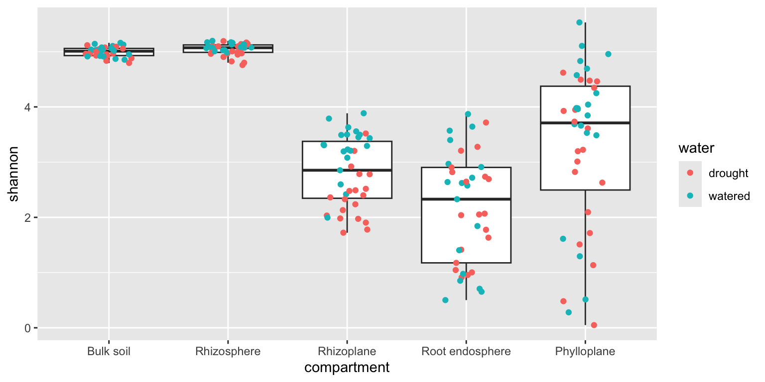
Which compartments differ from which? With five groups, that is a job for an ANOVA followed by a Tukey test (see the table in the theory part), in one line:
TukeyHSD(aov(shannon ~ compartment, data = alpha))One row per pair of compartments: diff is the difference of their means, p adj its p-value, corrected for the fact that you test ten pairs at once.
NoteCheckpoint
Bulk soil vs rhizosphere: p adj close to 1 (no difference). Rhizoplane vs phylloplane: 0.12. Every other pair: below 0.01. The spread is very different between compartments (look at the plot), which an ANOVA does not like: the table’s alternative, kruskal.test(shannon ~ compartment, data = alpha), reaches the same conclusion.
C3. Keep one compartment. Comparing climates across compartments would mix two very different questions. Work on one compartment at a time, starting with the rhizoplane:
rhizoplane <- alpha %>%
  filter(compartment == "Rhizoplane")

count(rhizoplane, water, heat, genotype)
NoteCheckpoint
39 samples, 8 combinations of water × heat × genotype, 4 or 5 samples each.
C4. Plot the design. The same kind of plot as for the biomass in B3:
ggplot(rhizoplane, aes(x = water, y = shannon, colour = heat)) +
  geom_boxplot(outlier.shape = NA) +
  geom_point(position = position_jitterdodge(jitter.width = 0.1)) +
  facet_wrap(~ genotype)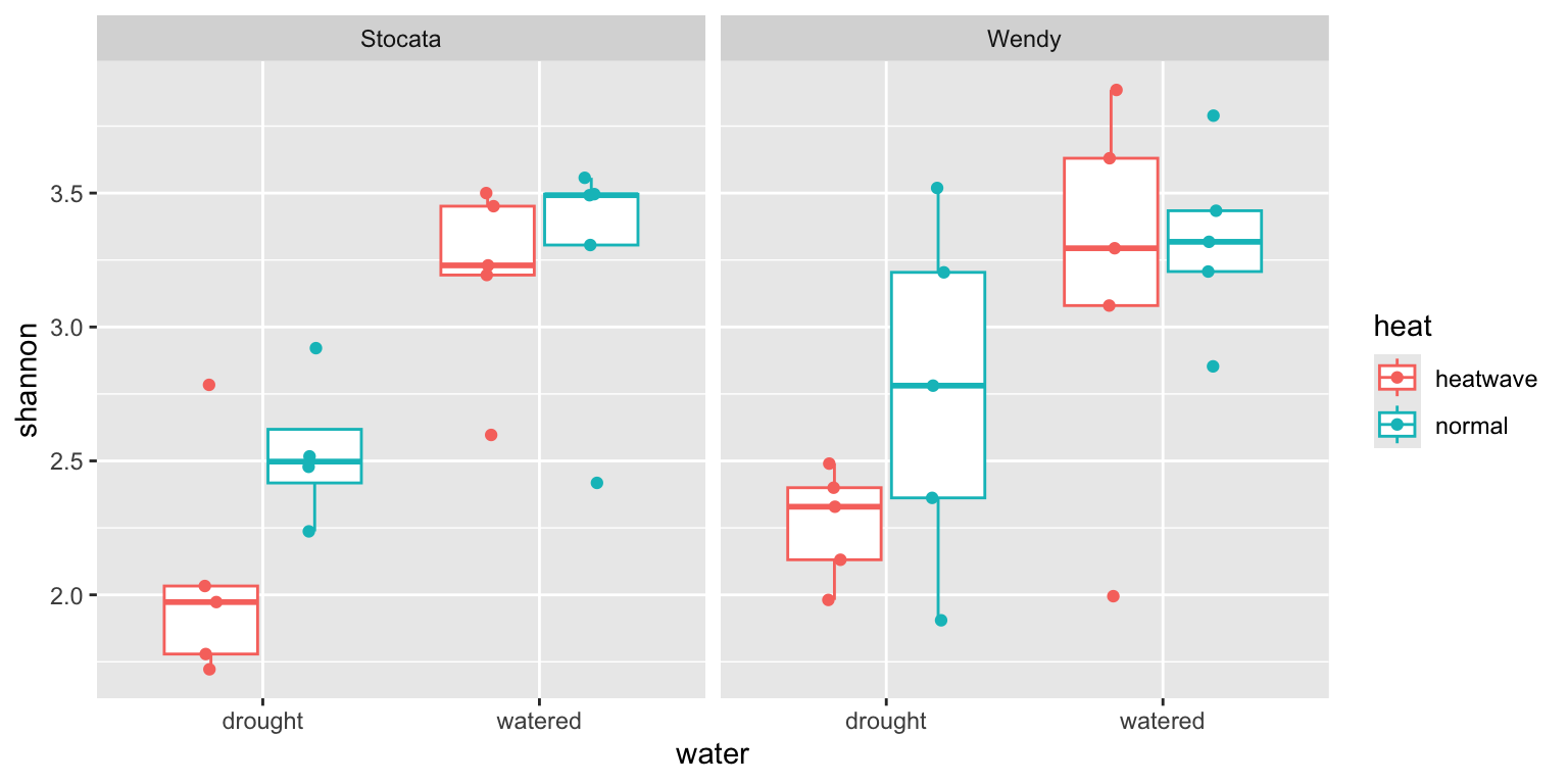
Before any statistics: which of the three factors seems to change Shannon diversity the most? Is it the same factor that weighed most on the plant’s biomass in B3? Write your guess in the workbook.
4.4.6 D. Guided: the statistics (16:15-16:35, pairs)
D1. Two groups: a t-test. Start with the simplest question: do watered and drought plants differ?
rhizoplane %>%
  group_by(water) %>%
  summarise(n = n(), mean_shannon = mean(shannon))

t.test(shannon ~ water, data = rhizoplane, var.equal = TRUE)
Read ~ as “explained by”: Shannon explained by water. var.equal = TRUE asks for the classic t-test, the one that assumes both groups vary as much.
NoteCheckpoint
Means of 2.40 (drought) and 3.24 (watered); the t-test gives p-value = 2.601e-06.
D2. The same test, as a linear model. Now fit lm() with the same formula, and read it with tidy() from the broom package (loaded in section A):
tidy(lm(shannon ~ water, data = rhizoplane))Two rows. (Intercept) is the mean of the drought plants (the reference group: first in alphabetical order). waterwatered is how much higher the watered plants are, and its p.value is exactly the t-test’s p-value. A t-test is a linear model with one factor: this is why the next step can simply add more factors.
D3. All three factors at once. One line fits water, heat, genotype and all their interactions; one more line splits the variation:
model_rhizoplane <- lm(shannon ~ water * heat * genotype, data = rhizoplane)
anova(model_rhizoplane)
Read the table row by row: one row per factor or interaction, Residuals last. The column Pr(>F) is the p-value; R adds stars to the small ones.
NoteCheckpoint
Only one row has three stars: water, with Pr(>F) = 4.01e-06. heat is close (0.06) but above 0.05. No interaction is significant.
D4. How much does each factor explain? The p-value says whether; the share of variation says how much. tidy() also turns the ANOVA table into a normal tibble, so you can compute with it:
anova_rhizoplane <- tidy(anova(model_rhizoplane)) %>%
  mutate(share = sumsq / sum(sumsq))
anova_rhizoplane

ggplot(anova_rhizoplane, aes(x = "Rhizoplane", y = share, fill = term)) +
  geom_col() +
  labs(x = NULL, y = "Share of variation in Shannon diversity")
One bar, cut into slices: the bigger the slice, the more that factor explains. The Residuals slice is everything the design does not explain.
NoteCheckpoint
water explains about 45% of the variation, the residuals about 45%, and everything else together about 10%.
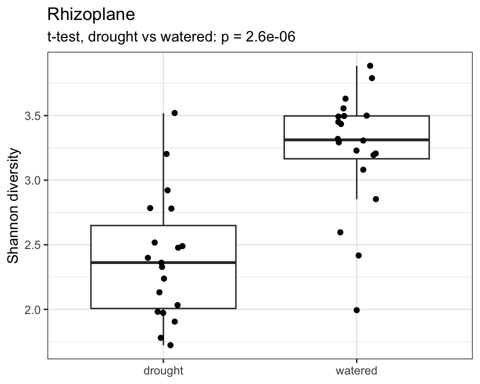
D5. Put the statistics on the plot. A figure should carry its own evidence. Keep the p-value in an object, then write it in the plot’s subtitle with paste(), which glues pieces of text together:
p_water <- t.test(shannon ~ water, data = rhizoplane, var.equal = TRUE)$p.value
p_water

ggplot(rhizoplane, aes(x = water, y = shannon)) +
  geom_boxplot(outlier.shape = NA) +
  geom_jitter(width = 0.1) +
  labs(title = "Rhizoplane",
       subtitle = paste("t-test, drought vs watered: p =", signif(p_water, 2)),
       x = NULL, y = "Shannon diversity") +
  theme_bw()
$p.value takes one element out of the test result. signif(p_water, 2) keeps two significant digits, so the subtitle reads p = 2.6e-06 instead of fifteen digits.
4.4.7 E. Alone: the bulk soil (16:35-16:55)
Now the bulk soil, the soil in the pot that does not touch the root. This time you do not redraw the same boxplot: you build a different kind of figure, an interaction plot, and put the statistics on it. Section E of the workbook guides you with a skeleton and a few ___ to fill.
What an interaction plot shows. One point per group mean, with an error bar (here the standard error: how precisely the mean is known), and a line joining the means of the same heat regime across the two water regimes. How to read it:
- a line that goes up or down: the water regime changes Shannon diversity;
- two lines far apart: the heat regime changes Shannon diversity;
- two lines that are not parallel: an interaction, the effect of drought depends on the heatwave.
You need three new geometries, all in the ggplot2 tab of the toolbox: geom_point() for the means, geom_line() to join them (with group = heat in aes(), so ggplot knows which points to join), and geom_errorbar() for the bars. The means and standard errors come from a group_by() + summarise(), as in B4.
Then, in the workbook:
- E1. Keep the bulk soil samples and count them (adapt C3).
- E2. Compute the means and standard errors, and draw the interaction plot.
- E3. Fit the three-factor model and compute the share of variation (adapt D3-D4).
- E4. Write the ANOVA p-values of heat and water on your plot (adapt D5), give it readable labels, and save it with
ggsave():
ggsave("results/bulk_soil_interaction.png", width = 6, height = 4)ggsave() saves the last plot drawn into results/. Then insert that file into your report yourself, below the chunk, as in the callout of block A: a caption of your own that says what the figure shows, the label #fig-bulk, a width of 80%. Cite it as @fig-bulk in your answer to E5. Then answer the E questions: they are the graded part of today. Compare with the rhizoplane: is the answer the same? Is the most significant effect also a large one, in Shannon units? Look at the y axis of your plot before you answer.
4.4.8 Wrap-up (16:55-17:00)
Click Render one last time. Check that WORKBOOK.html shows your bulk soil figure and your ANOVA table, and that results/bulk_soil_interaction.png exists. You can finish the written answers at home: submit WORKBOOK.html on Moodle by Sunday evening (18 October). Your workbook file still says “Thursday” at the top: the date on this page is the right one.
If your workbook refuses to render at the end, do not panic: submit WORKBOOK.qmd instead, and say in the last section where it fails.
NoteHow this is graded (10 points)
| Criterion | Points | What it looks for |
|---|---|---|
| Reproducible workflow | 2 | The workbook renders (or the code is complete and in order), inside a clean project. |
| Working analysis | 3 | Sections A-E ran and the checkpoint numbers you copied are right. |
| Required result | 2 | The bulk soil interaction plot (section E): means, error bars, readable labels, the p-values written on it, saved and inserted into the report with a caption. |
| Biological interpretation | 2 | Your answer to E5, citing your own numbers and comparing the bulk soil with the rhizoplane. |
| Reflection | 1 | Your limitation sentence in E6. |
4.5 Checkpoint
You are done when all of the following are true:
- your
session_04folder is an R project withdata/,results/and a workbook that renders; - you can explain the design of the experiment from your map: the conditions, why they are mixed in space, and why each plant had one job;
- you can say how much drought and the heatwave reduced the plants’ biomass, and which organ suffered most;
- you can say what a row and a column of
alpharepresent, and why some compartments have fewer than 40 samples; - you used
filter,mutate,count,group_by+summariseandpivot_longer, and can say in one sentence what each one did; - you built a ggplot with boxes, points, colours and facets, a map with
geom_tile(), and an interaction plot with means, lines and error bars; - you used a Tukey test to find which compartments differ, and know which test to pick for a new question from the table;
- you ran a t-test and found the same p-value with
lm(); - you fitted
lm(shannon ~ water * heat * genotype)on two compartments and can say, for each, which factor matters and how much of the variation it explains; - you wrote a p-value on a plot from a value computed in R, not typed by hand;
- you inserted a saved figure into your report, with a caption, and cited it with
@fig-bulk; - you can explain why a significant effect is not necessarily a large one.
4.6 Optional challenge
For your own interest, not graded.
A. All five compartments in one figure. Repeat D3-D4 for the rhizosphere, the root endosphere and the phylloplane, add a compartment column to each anova_... table with mutate(), stack them with bind_rows(), and draw one bar per compartment with geom_col(). Is there a pattern from soil to leaf?
B. Check the model’s assumptions. A linear model assumes the residuals are roughly normal and equally spread across groups. plot(model_rhizoplane, which = 1) and plot(model_rhizoplane, which = 2) draw the two classic diagnostic plots. Do the rhizoplane residuals look acceptable?
C. The plant is not independent. The rhizoplane and the root endosphere come from the same plants (look at the plant column). Fitting one model on both compartments at once, with the plant as a random effect, is what a mixed model does: lme4::lmer(shannon ~ compartment * water + (1 | plant), data = ...). What changes compared to two separate models?
D. Does the place in the experiment matter? Colour the map by biomass instead of water regime, with one panel per climate so that the drought effect does not hide everything else:
ggplot(physio, aes(x = position, y = line, fill = biomass_total)) +
  geom_tile() +
  facet_grid(heat ~ water)
Do the plants at one end of the lines, or on one line, look bigger? Then test it: add + line + position at the end of a model of biomass_total. Why does the mixing you saw in B2 protect the conclusions even if position has a small effect?
E. Two stresses together. Fit lm(biomass_total ~ water * heat * genotype, data = physio), look at its ANOVA table, then fit the same model on log(biomass_total). The interaction water:heat changes a lot. Compute, from B4, by how many percent the heatwave reduces the biomass of watered plants, and of drought plants. What does the log scale see that the raw scale missed, and what does it mean for a plant facing both stresses at once?
4.7 Going further
Free, well-written references if you want more statistics than one session can hold:
- Common statistical tests are linear models (J. K. Lindeløv): t-test, ANOVA, correlation… all as
lm(), with R code. - Points of Significance (Nature Methods, free access): two-page articles for biologists, in particular Two-factor designs.
- Data Carpentry: R for Ecologists: a complete beginner course on R, dplyr and ggplot2.
- Introduction to Statistics with R (SIB Swiss Institute of Bioinformatics).
4.8 Before the next session
Session 5 moves from one variable (Shannon diversity) to hundreds at once: a metabolomics table, where every column is a molecule. You will keep the same R project habits, the same dplyr verbs and ggplot layers, and meet two new kinds of plots to see the whole table in one picture.
4.9 Answers
NoteOpen this after you have tried the exercises yourself
Session 4 has now been submitted. Below are the real answers, computed with the exact workbook code on LEGcompute: use them to check your own reasoning, not to replace it. Small rounding differences (second decimal) are normal.
A1. The plant table. 240 rows, 12 columns. One row is one plant of the final harvest. NA in the biomass columns: the plant was not weighed, because it was used for another job (omics and soil, plant microbiome), or the measure failed.
B1. Plants per job. 66 physiology, 53 exudates, 75 omics_and_soil, 46 plant_microbiome. The rhizoplane bacteria come from the plant_microbiome plants; the bulk soil bacteria from the soil of the omics_and_soil plants.
B2. The map. The conditions are mixed: watered and drought rhizotubes, and the two cultivars, alternate along the lines. Mixing on purpose (randomisation) prevents a place effect (light, draught, the edge of the bench) from being mistaken for a treatment effect. The two maps have exactly the same layout: the same randomisation plan was used for both heat regimes.
B4. Biomass per climate. 108 plants weighed.
| water | heat | n | mean_biomass (g) |
|---|---|---|---|
| drought | heatwave | 25 | 0.32 |
| drought | normal | 24 | 0.50 |
| watered | heatwave | 27 | 1.16 |
| watered | normal | 32 | 1.25 |
Drought weighs far more: it divides the biomass by more than two. The heatwave removes a little more on top: about 7% of the biomass of watered plants, but 35% of drought plants (see optional challenge E).
B5. Per organ. 324 rows = 108 plants × 3 organs. Mean biomass, watered → drought: leaf 0.61 → 0.19 g (−68%), stem 0.39 → 0.13 g (−66%), root 0.21 → 0.08 g (−61%). The root keeps the largest share of its biomass (its share of the total rises from 18% to 20%): keeping roots helps the plant explore the soil for the little water left.
C1. The bacteria table. Rhizoplane (39), rhizosphere (39) and root endosphere (37) have fewer than 40 samples: 5 compartments × 40 plants = 200 expected, 195 present, 5 missing.
C2. Diversity per compartment.
| Compartment | n | mean_shannon | sd_shannon |
|---|---|---|---|
| Bulk soil | 40 | 5.00 | 0.088 |
| Rhizosphere | 39 | 5.05 | 0.104 |
| Rhizoplane | 39 | 2.83 | 0.631 |
| Root endosphere | 37 | 2.17 | 0.999 |
| Phylloplane | 40 | 3.28 | 1.46 |
Most diverse: rhizosphere and bulk soil (about 5). Least: root endosphere (about 2.2). Tukey: only two pairs do not differ, Rhizosphere-Bulk soil (p adj = 0.9988) and Phylloplane-Rhizoplane (0.1206); Root endosphere-Rhizoplane 0.0072, all the others below 0.0001. Why fewer bacteria inside the root: the root is a filter. Few soil bacteria can cross the root surface and live inside the tissues; the plant’s immune system and the chemistry inside the root select a small, specialised community.
C3. The rhizoplane. 39 samples, 8 combinations, 5 each except drought × normal × Stocata (4).
C4. Your guess. Water, the factor that weighed most on biomass: checked in D4.
D1. t-test. Watered 3.24, drought 2.40 (a drop of 0.84 Shannon units). t = −5.54, df = 37, p-value = 2.601e-06.
D2. The same test as a linear model. (Intercept) 2.40 is the drought mean; waterwatered 0.839 is the difference between the two means (3.24 − 2.40). Its p-value, 2.60e-06, is identical to the t-test’s: a t-test is a linear model with one factor.
D3. Three factors at once. Only water is below 0.05: Pr(>F) = 4.01e-06. heat 0.060, genotype 0.43, no interaction below 0.2. (If you changed the order of the factors in the formula, heat can come out at 0.046: with this design, the order matters a little.)
D4. Share of variation. Water 45.4%, residuals 45.1%, heat 5.5%, water:heat 2.4%, everything else below 1% each. Your C4 guess (water) was right.
D5. The p-value on the plot. t-test, drought vs watered: p = 2.6e-06. Computed in R, not typed: no typing error, and it updates by itself if the data or the test change.
E. The bulk soil, the code. One way to write it:
# E1
bulk_soil <- alpha %>%
  filter(compartment == "Bulk soil")
count(bulk_soil, water, heat, genotype)

# E2
bulk_soil_means <- bulk_soil %>%
  group_by(water, heat) %>%
  summarise(mean_shannon = mean(shannon),
            se = sd(shannon) / sqrt(n()))

plot_bulk_soil <- ggplot(bulk_soil_means,
                         aes(x = water, y = mean_shannon, colour = heat, group = heat)) +
  geom_point(size = 3) +
  geom_line() +
  geom_errorbar(aes(ymin = mean_shannon - se, ymax = mean_shannon + se), width = 0.1)

# E3
model_bulk_soil <- lm(shannon ~ water * heat * genotype, data = bulk_soil)
anova_bulk_soil <- tidy(anova(model_bulk_soil)) %>%
  mutate(share = sumsq / sum(sumsq))

# E4
p_heat  <- anova_bulk_soil %>% filter(term == "heat") %>% pull(p.value)
p_water <- anova_bulk_soil %>% filter(term == "water") %>% pull(p.value)

plot_bulk_soil +
  labs(title = "Bulk soil",
       subtitle = paste("ANOVA: heat p =", signif(p_heat, 2),
                        "| water p =", signif(p_water, 2)),
       x = "Water regime", y = "Mean Shannon diversity (± SE)", colour = "Heat regime") +
  theme_bw()

ggsave("results/bulk_soil_interaction.png", width = 6, height = 4)
Then, below the chunk, the image line:
{#fig-bulk width=80%}E1. 40 samples, 5 per combination (fully balanced).
E2. Means: drought × heatwave 4.91, drought × normal 5.05, watered × heatwave 4.97, watered × normal 5.06 (SE about 0.02). Heat moves the means the most: the two lines are far apart, while each line is almost flat from drought to watered. The lines are roughly parallel: no clear interaction. Non-parallel lines would mean that the effect of drought depends on the heat regime.
E3. Only heat is significant: Pr(>F) = 1.45e-05, 42.0% of the variation. Water 3.2% (p = 0.17), genotype 1.1%, no significant interaction (water:heat p = 0.35), residuals 51.5%. The heatwave lowers diversity by about 0.1 Shannon units, against 0.84 for drought on the rhizoplane: about eight times smaller.
E4. Your figure should look like this one, and appear as Figure 2:
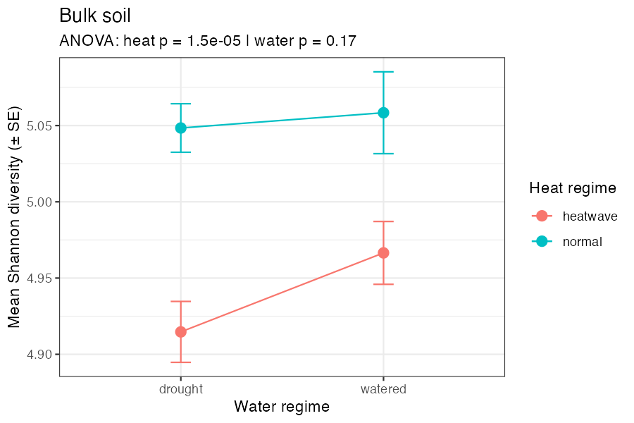
Look at the y axis: it runs from about 4.90 to 5.07. ggplot zooms in, so a difference of 0.1 looks as large as the 0.84 of the rhizoplane.
E5. A complete answer.
In the bulk soil, drought does not change bacterial diversity (p = 0.17, 3% of the variation), whereas the heatwave lowers it slightly (from about 5.05 to 4.94, p = 1.5e-05, 42% of the variation; Figure 2). On the rhizoplane it is the opposite: drought is the main factor (3.24 to 2.40, p = 4e-06, 45% of the variation) and the heatwave is not significant. Drought probably acts through the plant: a thirsty root changes what it releases and how much water it draws right at its surface, while the soil further away hardly feels it. The bulk soil heatwave effect is highly significant but tiny (about 0.1 Shannon units, against 0.84 for drought on the rhizoplane): bulk soil samples vary so little that even a small difference stands out.
The key idea: significant is not large. A very small p-value says the difference is unlikely to be chance, not that it matters biologically.
E6. Good limitations. The bulk soil effect is significant but very small, and the zoomed y axis makes it look large; only 5 plants per combination; Shannon is one number and says nothing about which bacteria changed; biomass and bacteria come from different plants, so no plant-by-plant link is possible; one experiment, one season; the model’s assumptions were not checked; several compartments and many tests, so some p-values below 0.05 can appear by chance.
Optional challenge A. The two main factors, compartment by compartment:
| Compartment | water: p (share) | heat: p (share) |
|---|---|---|
| Bulk soil | 0.17 (3%) | 1.5e-05 (42%) |
| Rhizosphere | 0.019 (15%) | 0.49 (1%) |
| Rhizoplane | 4.0e-06 (45%) | 0.060 (6%) |
| Root endosphere | 0.65 (0.4%) | 0.074 (6%) |
| Phylloplane | 0.085 (5%) | 0.0023 (16%) |
A pattern from soil to leaf: drought matters more and more as you come closer to the root surface (bulk soil 3%, rhizosphere 15%, rhizoplane 45%), but not inside the root, where the plant filters its bacteria. The heatwave matters where the bacteria are exposed to the air temperature: the bulk soil and the leaf surface.
Optional challenge B. The rhizoplane residuals look acceptable: no clear trend or funnel on the first plot, points close to the line on the second (Shapiro test p = 0.25), and a similar spread in both water regimes (sd 0.48 under drought, 0.46 watered).
Optional challenge C. 36 of the 40 plants have both a rhizoplane and an endosphere sample. In the mixed model, the plant effect has a standard deviation of 0.42, against 0.66 for the residuals: about 28% of the remaining variation is shared by the two compartments of the same plant. Two separate models treat these samples as independent, which they are not. The conclusion does not change: drought lowers the rhizoplane (+0.83 when watered) but hardly the endosphere (the compartment:water interaction, −0.70, cancels most of it: t = −2.28).
Optional challenge D. With one panel per climate, no obvious gradient appears. Added after the treatments, line p = 0.52 and position p = 0.07: no clear place effect. Even if position had a small effect, the mixing protects the conclusions: any place effect is spread over all conditions instead of piling up on one.
Optional challenge E. Raw scale: water:heat p = 0.22. Log scale: water:heat p = 1e-5. From B4, the heatwave removes about 7% of a watered plant’s biomass (1.25 → 1.16 g) but 35% of a drought plant’s (0.50 → 0.32 g). A log scale compares ratios, not differences: in relative terms, the two stresses together hurt more than the sum of each alone. That is how a plant biologist usually thinks about growth.