3 Session 3: Sequence similarity and phylogeny
3.1 Overview
Download the lecture slides (PDF)
Respond at pe.app/cmaslard2
You are handed one unidentified sequence. Which of a handful of reference sequences is it most similar to, and what does that similarity tell you about where it came from?
Sessions 1 and 2 taught you to look inside a sequence file and to judge whether its reads can be trusted. Today’s question is different: given one sequence on its own, how do you work out what it is related to? That is the question behind every “what is this?” moment in biology, from identifying a contaminant in a culture to tracing the origin of a new virus. You will run two similarity searches of increasing sensitivity, inspect a real alignment and a distance matrix by hand, build and annotate a real phylogenetic tree, and cross-check your conclusion at the protein level, all on sequences from a family of viruses everyone in the room has lived through.
Sessions 1 and 2 were not graded. From today, every session ends with a short individual, graded task. Today’s required result is one annotated tree, saved as an image, with a written biological interpretation. You draft that interpretation in class, in Section 5 of WORKSHEET.md, but you have until Thursday to polish it and submit: see the rubric below, in the wrap-up section.
3.1.1 Learning outcomes
By the end of this session, you should be able to:
- explain what a similarity search reports (percent identity, alignment length, E-value, bit score) and roughly what each number means, including why they can disagree with each other on which hit is “best”;
- run
blastnat two different sensitivity settings against a small prepared reference database, and read the output table; - explain, in plain language, how a multiple alignment turns into a phylogenetic tree, and read a distance matrix as a table;
- read a rooted tree: tip, internal node, branch length, clade, outgroup, support value;
- fetch real sequences from NCBI yourself, align and build a tree from them with MAFFT and FastTree, then plot it in R and edit one part of the script to test what rerooting does and does not change;
- cross-check a nucleotide-level conclusion with a protein-level search on the same genes;
- state a biological conclusion about an unknown sequence, backed by more than one kind of evidence, and name one limitation of that conclusion.
3.1.2 Session plan
| Time | Block | What happens |
|---|---|---|
| 14:15-14:20 | Retrieval | One question from Session 2, then today’s question. |
| 14:20-14:35 | Theory 1 | Similarity search: what BLAST actually measures. |
| 14:35-14:50 | Theory 2 | From alignment to tree; worked example; two-minute UniProt detour. |
| 14:50-15:00 | Practical briefing | What “which reference is closest?” will ask of you today. |
| 15:00-15:15 | Practical A | Rebuild the project folder, fetch the sequences. |
| 15:15-15:35 | Practical B | Two BLAST searches: quick, then deep. |
| 15:35-15:50 | Practical C | Inspect a prepared alignment and distance matrix by hand. |
| 15:50-16:00 | Checkpoint | Both searches done, alignment and matrix read. Short break. |
| 16:00-16:40 | Practical D | Fetch real NCBI data, align with MAFFT, build the tree with FastTree, plot and annotate in R. (pairs) |
| 16:40-16:50 | Practical D2 | Same question, at the protein level. (pairs) |
| 16:50-17:00 | Practical E | Draft your interpretation; polish and submit by Thursday. |
3.2 Theory (≈45 min)
3.2.1 1. Similarity search: what BLAST actually measures
grep (Sessions 1-2) finds exact text. Biological sequences almost never match exactly: mutation, sequencing error, and evolutionary divergence all change a handful of bases here and there. BLAST (Basic Local Alignment Search Tool) finds sequences that are similar enough, scores how similar, and does it against thousands of sequences at once, in seconds.
Given one query sequence and a set of reference sequences, blastn reports one row per match it considers meaningful:
| Column | Meaning |
|---|---|
pident |
percent identity: of the aligned bases, what fraction are identical |
length |
how many bases the alignment covers |
evalue |
how many matches this good would be expected by chance alone; smaller is better, 0.0 means effectively impossible by chance |
bitscore |
an overall match quality score, normalized so it is comparable between searches; higher is better |
A high pident over a short length can still be a coincidence; a lower pident over a long length with a tiny evalue usually is not. Reading a BLAST hit means looking at these together, not just the percent identity on its own. Block B gives you a real case where trusting pident alone would mislead you.
Session 1’s mystery.fasta contained one record, sp|P0DTC2|SPIKE_SARS2, that was neither obviously DNA nor identifiable by eye. A similarity search is exactly the next step you would take on a record like that: not “does it look like DNA”, but “what does it match”. You meet that exact sequence again at the end of this theory block.
Search settings matter, too. BLAST can run in a fast, strict mode tuned for near-identical sequences, or a slower, more sensitive mode that also reports weaker, more distant matches. Neither is “wrong”; they answer slightly different questions, and today’s practical uses both, deliberately, one after the other.
3.2.2 2. From one match to a tree
BLAST answers “what is my sequence most similar to”, one hit at a time. A phylogenetic tree goes further: it places every sequence you give it, including ones too different from each other for a strict BLAST search to confidently match, on a single diagram of relative relatedness. Three steps get you there:
- Multiple sequence alignment. Every sequence is stacked and padded with gaps (
-) so that the same column means the same position in every sequence. Session 2’s FASTQ lines were already the same length by construction; here, alignment is the step that creates that correspondence across sequences that differ in length. - Distance. Once sequences line up column by column, counting the fraction of columns that differ between every pair of sequences gives a distance: more differences, more distant. Doing this for every pair at once gives a distance matrix, one number per pair; today you will read it as a table, the same idea scales to a colour-coded heatmap for larger datasets than today’s.
- Tree building. An algorithm arranges sequences on a tree so that closely related sequences sit together, joined by a recent common node. Today’s tool, FastTree, does this quickly even for larger alignments than ours, using a statistical (approximately maximum-likelihood) model rather than the distance matrix alone, and it reports a support value at each split: roughly, how confident the method is that this grouping is real rather than an artefact of this particular alignment.
| Term | Meaning |
|---|---|
| Tip | one sequence, labelled, at the end of a branch |
| Node | a point where branches split: the inferred common ancestor of everything beyond it |
| Branch length | genetic distance (not necessarily time) between a node and the sequence or node it leads to |
| Clade | a node plus everything descended from it: a complete sub-group |
| Outgroup | a sequence known to be the most distantly related, used to anchor which end of the tree is the root |
| Support value | confidence (here, 0 to 1) that a given split is real, from resampling the alignment many times and checking how often the same split reappears |
Two tips drawn close together are closely related because of where their shared node is, not because they happen to be printed near each other. Always trace back to the node.
FastTree’s speed comes from heuristics, not from skipping statistics: it is a fast, reasonable first answer, not the last word on a dataset this size. One known weakness, relevant for today’s most distant sequences: raw percent-difference, the simplest possible distance, underestimates true evolutionary distance once enough time has passed for the same site to mutate more than once (“saturation”). Distance correction models (for example Jukes-Cantor) attempt to account for this. A full, maximum-likelihood tree with properly resampled bootstrap support (rather than FastTree’s faster approximation) is the published standard, and out of scope for today, but the optional challenge lets you try a correction model on today’s data.
3.2.4 Practical briefing
You will fetch one unidentified sequence (unknown_sample.fasta) and four named reference sequences, all spike genes from different coronaviruses. You will BLAST the unknown against the references yourself, at two sensitivity settings, inspect a prepared alignment and distance matrix by hand, render and annotate a prepared tree in R, and finally repeat the comparison at the protein level. Everything you run goes in your command log, exactly like Sessions 1-2.
3.3 Practical (≈1 h 50)
3.3.1 New commands for today
Eleven new commands on top of everything from Sessions 1-2: today’s practical went well past this course’s usual limit of six, on purpose, because block D now has you fetch real data from NCBI yourselves rather than start from a prepared file. Treat esearch/efetch as one pattern, the same way you already treat module load X as one pattern, and this is closer to nine ideas than eleven.
| Command | What it does | Example |
|---|---|---|
module load BLAST+ |
make the BLAST programs available in this session | module load BLAST+ |
makeblastdb |
turn a FASTA file into a searchable database | makeblastdb -in refs.fasta -dbtype nucl -out refs_db |
blastn |
search a nucleotide query against a nucleotide database | blastn -query q.fasta -db refs_db -outfmt 6 |
blastp |
search a protein query against a protein database | blastp -query q.fasta -db refs_db -outfmt 6 |
esearch / efetch |
search and download real records from NCBI | esearch -db nucleotide -query "..." \| efetch -format fasta |
mafft |
align a set of unaligned sequences | mafft --auto in.fasta > aligned.fasta |
FastTree |
build a tree from an aligned FASTA file | FastTree -nt aligned.fasta > tree.nwk |
sed |
search and replace text in a file | sed -i "s/old/new/" file.fasta |
pip install --user / clipkit |
install a small Python tool into your own account, then run it | pip install --user clipkit |
| (RStudio) Source | run an entire R script from the Console or the Source button | source("plot_tree.R") |
module load BLAST+ resolves to the current default, BLAST+/2.17.0-gompi-2025b, module load FastTree to FastTree/2.2-GCCcore-13.3.0, module load EntrezDirect to EntrezDirect/24.4.20250710, and module load MAFFT to MAFFT/7.526-GCC-14.2.0-with-extensions: the same module load X pattern as SAMtools and FastQC in Sessions 1-2. ClipKIT is not a cluster module (there is none): module load Python then python3 -m pip install --user clipkit installs it in a few seconds, confirmed working. The R step needs no module load at all: RStudio Server’s R already has ape installed.
3.3.2 A. Rebuild the project and fetch the data (15:00-15:15)
Reopen bioinfo_course from Sessions 1-2. Predict each line before running it.
cd ~/bioinfo_course
mkdir session_03
cd session_03
mkdir data results
cd data
pwdpwd ends in bioinfo_course/session_03/data. Same two-folder habit as Session 2: raw input in data, everything you generate in results.
Copy in today’s sequences, the prepared alignment and tree, the R script, and your worksheet:
cp /home/cmaslard/bioinfo_tools_course/session_03/unknown_sample.fasta .
cp /home/cmaslard/bioinfo_tools_course/session_03/reference_spike_genes.fasta .
cp /home/cmaslard/bioinfo_tools_course/session_03/reference_spike_proteins.fasta .
cp /home/cmaslard/bioinfo_tools_course/session_03/aligned_spike.fasta .
cp /home/cmaslard/bioinfo_tools_course/session_03/sars_variants_aligned.fasta .
cp /home/cmaslard/bioinfo_tools_course/session_03/sars_variants_tree.nwk .
cp /home/cmaslard/bioinfo_tools_course/session_03/plot_tree.R .
cp /home/cmaslard/bioinfo_tools_course/session_03/WORKSHEET.md .
ls -lh
unknown_sample.fasta is the sequence you are identifying today. reference_spike_genes.fasta and reference_spike_proteins.fasta hold the same four coronaviruses’ spike genes, as nucleotide and as protein, to compare it against. aligned_spike.fasta is prepared: the alignment is already built for you, from the same five nucleotide sequences, so that block C starts from a correct result, instead of spending the whole afternoon on alignment software. sars_variants_aligned.fasta and sars_variants_tree.nwk are fallbacks for block D, where you fetch and build your own much larger tree from live NCBI data: if the live fetch, MAFFT, or FastTree runs into trouble, these let you continue from a known-good point; tell your instructor if you need to fall back to them.
grep "^>" reference_spike_genes.fastaFour headers: SARS-CoV-2_Wuhan-Hu-1, SARS-CoV-1_Tor2, MERS-CoV, HCoV-OC43_seasonal. unknown_sample.fasta has exactly one record, unknown_sample, and no clue in its header about which of the four it belongs with.
3.3.3 B. Two searches, quick then deep (15:15-15:35)
module load BLAST+
makeblastdb -in reference_spike_genes.fasta -dbtype nucl -out ../results/spike_db
blastn -query unknown_sample.fasta -db ../results/spike_db -outfmt 6 -out ../results/blast_result.tsv
cat ../results/blast_result.tsv
-outfmt 6 requests a plain tab-separated table, in this column order:
qseqid sseqid pident length mismatch gapopen qstart qend sstart send evalue bitscoreblast_result.tsv has exactly one line: unknown_sample against SARS-CoV-2_Wuhan-Hu-1, at roughly 93% identity over essentially the whole gene (length ≈ 3,800), with evalue 0.0. Only one reference produced a hit at all under these default (strict) search settings; the other three did not even appear in the table.
A strict search can tell you “nothing” about a real relationship, not because there is none, but because the match fell below what the search was tuned to report. Run a second, more sensitive search against the same database:
blastn -query unknown_sample.fasta -db ../results/spike_db -task blastn -evalue 1e-3 -max_hsps 1 -outfmt 6 -out ../results/blast_result_deep.tsv
cat ../results/blast_result_deep.tsv
-task blastn switches from the strict default algorithm to the standard, more sensitive one; -evalue 1e-3 relaxes how significant a match must be to get reported; -max_hsps 1 keeps only each reference’s single best-scoring match.
This time, blast_result_deep.tsv has four lines, one per reference. Look closely at length, evalue, and bitscore, not just pident, for the two weakest hits (MERS-CoV and HCoV-OC43_seasonal). One of the two has a higher pident than the other, but a shorter length, a weaker evalue, and a lower bitscore. Which one actually looks like the better-supported match, and why? Write your answer in Section 2 of your worksheet: this is the real case the theory block warned you about.
3.3.4 C. Inspect the alignment and the distance matrix (15:35-15:50)
head -5 aligned_spike.fastaEvery sequence in aligned_spike.fasta is now exactly the same length (4,551 columns), padded with - where an insertion in one sequence has no counterpart in another. That is what “aligned” means: column 1,000 is the same position in every sequence on the file.
Below is one 60-column window of that same alignment (columns 411-470), already extracted for you:
SARS-CoV-2_Wuhan-Hu-1   tcgaagacccagtccctacttattgttaataacgctactaatgttgttattaaagtctgt
unknown_sample          tcgaagacccagtctctacttattgttaataacgctactaatgttgttattaaagtctgt
SARS-CoV-1_Tor2         aacaagtcacagtcggtgattattattaacaattctactaatgttgttatacgagcatgt
MERS-CoV                gccaattccactggcactgttattattagcccatctaccagcgctactatacgaaaaatt
HCoV-OC43_seasonal      gctataactataggtagtacttttgtaaatacatcctatagtgtggtagtacaaccacgt
By eye, count how many of the 60 positions in unknown_sample differ from each reference in this window. Write the four counts in Section 3 of your worksheet.
Now compare your small-window counts with the whole-alignment picture, all 4,551 columns, already computed for you as a percent difference from unknown_sample:
| Reference | % different from unknown_sample, whole gene |
|---|---|
| SARS-CoV-2_Wuhan-Hu-1 | 6.9% |
| SARS-CoV-1_Tor2 | 25.7% |
| MERS-CoV | 51.3% |
| HCoV-OC43_seasonal | 50.8% |
Counting one reference carefully in the 60-column window and estimating the rest (“clearly close”, “clearly different”) is enough; the whole-gene table above is given to you either way.
Your 60-column window, block B’s deep search, and this whole-gene table should mostly agree on the overall order: SARS-CoV-2 closest, SARS-CoV-1 next, then MERS-CoV and HCoV-OC43_seasonal far behind both. Look closely, though, at which of the last two is more distant according to this table, versus according to block B’s bitscore. Note whether they agree in Section 3 of your worksheet: a real disagreement between two reasonable methods, on the two hardest-to-place sequences, is normal, not a mistake, and exactly the kind of limitation worth naming in Section 5.
3.3.5 15:50-16:00: Checkpoint and short break
Before you step away: both blast_result.tsv and blast_result_deep.tsv exist, you have counted mismatches in the alignment window and read the whole-gene table, and your script is saved.
3.3.6 D. Fetch real NCBI data and build a tree, for real (16:00-16:40, pairs)
So far every file has been prepared for you. For this one block, you fetch the sequences yourselves, straight from NCBI, and build a tree from data nobody has cleaned up for you first. You will also add unknown_sample into this much bigger tree: does it land inside the real SARS-CoV-2 diversity, or outside it, as its own separate branch? This is an independent check on blocks B-D2’s conclusion, by a completely different method.
This block has more to do than today’s others, on purpose, now that you are working with a real public database instead of a prepared file. It is fine if you do not finish everything before 16:40: get the tree itself built and plotted first, that is the required part; the questions below it in WORKSHEET.md can be finished before Thursday, the same as Section 5.
First, see how big this search really is, before limiting it to something you can download in a few minutes:
export NCBI_API_KEY=a47f27d793c7483a1c90f4d38c29c62a9d08
module load EntrezDirect
esearch -db nucleotide -query "Severe acute respiratory syndrome coronavirus 2 isolate SARS-CoV-2"
The first line sets an environment variable, NCBI_API_KEY, the same idea as $PATH or any other variable, just one NCBI’s tools look for by name. Registering this key with NCBI (already done for the whole class) raises how many requests per second you are allowed to make to their servers, from 3 to 10 — useful with everyone in the room querying around the same time. esearch -db nucleotide -query "..." is the actual search: -db nucleotide says which NCBI database to search, -query is the search term, the same kind of text you could type into NCBI’s website search box.
Everyone using the same key above means everyone shares its 10-requests-per-second allowance, not 10 each. If you want, get your own, free, in under a minute: NCBI account → Settings → API Key Management → Create an API Key, then replace the key on the first line with yours instead. Entirely optional, but if the fetch feels slow with everyone running it at once, this is the first thing to try.
This prints a short block of XML to the screen; the <Count> line is how many matching records exist on NCBI right now, out of all SARS-CoV-2 genomes ever submitted. Note it down: this is not how many you are about to download.
Now fetch a manageable subset: 100 of those, plus 13 specific named variants by accession, plus unknown_sample itself, already sitting in your data folder since block A:
esearch -db nucleotide -query "Severe acute respiratory syndrome coronavirus 2 isolate SARS-CoV-2" | efetch -format fasta -stop 100 > sars_variants.fasta
efetch -db nuccore -id MN908947.1,MW931310.1,OU297363.1,OK252993.1,MZ727692.1,OX315743.1,OX315675.1,OP093374.1,OP164778.1,OP457109.1,PP997352.1,PQ325441.1,PQ356432.1 -format fasta >> sars_variants.fasta
cat unknown_sample.fasta >> sars_variants.fasta
grep -c ">" sars_variants.fasta
The first line reuses the same esearch search as above, but this time pipes (|) its result into efetch, the same search → fetch pattern as esearch | efetch anywhere else today: esearch finds matching records, efetch downloads them. -format fasta asks for plain FASTA, the format you already know; -stop 100 caps it at the first 100 results, since efetch would otherwise try to download every one of the millions you just counted. -stop 100 is a time budget, not a hard limit: if you are ahead and curious, you can rerun this line with a bigger number (-stop 300, say) before moving on — MAFFT and FastTree both take longer with more sequences, so check the time before committing to a much larger number. The second line is a different pattern: efetch -db nuccore -id ACC1,ACC2,... fetches specific, known accessions directly, no esearch needed first, because you already know exactly which 13 records you want, listed by accession and separated by commas. >> (two angle brackets, not one) appends to the file instead of overwriting it, so this line adds its 13 sequences onto the 100 already in sars_variants.fasta rather than replacing them; the third line, a plain cat, appends unknown_sample.fasta the same way:
| Accession | Variant | Accession | Variant |
|---|---|---|---|
MN908947.1 |
Wuhan-Hu-1 (the original reference) | OP164778.1 |
Omicron BA.5 |
MW931310.1 |
Delta | OP457109.1 |
Omicron BA.2.75 |
OU297363.1 |
Alpha | PP997352.1 |
Omicron 24A |
OK252993.1 |
Gamma | PQ325441.1 |
Omicron 24B |
MZ727692.1 |
Mu | PQ356432.1 |
Omicron 24C |
OX315743.1 |
Omicron BA.1 | OX315675.1 |
Omicron BA.2 |
OP093374.1 |
Omicron BA.4 |
sars_variants.fasta has 114 sequences. You will likely see a red-looking line starting curl: (56) OpenSSL SSL_read... during the fetch: this is a benign, known quirk of this network path, not a failure. esearch/efetch retry automatically and the file still ends up correct; check the count above before worrying about it. unknown_sample is much shorter than the 113 full genomes (it is only the spike gene region): expect it to look mostly gaps (-) if you peek at the alignment later, that is expected, not a problem.
Before aligning, look up one real record in more detail. FASTA only gives you a sequence and a one-line header; NCBI’s full GenBank format carries structured metadata too:
efetch -db nuccore -id MN908947.1 -format gb | grep "geo_loc_name\|collection_date\|isolate="Three lines: the isolate name, where the sample was collected, and when. Write both down in Section 4 of WORKSHEET.md. This is the earliest known SARS-CoV-2 genome sequenced: every other sequence in your tree is, directly or indirectly, a descendant of this one.
Align, then build the tree, the same module load pattern you already used for BLAST+ in block B, and will use again for FastTree below:
module load MAFFT
mafft --auto --thread 8 sars_variants.fasta > ../results/sars_variants_aligned_mine.fasta
--auto lets MAFFT pick its own alignment strategy based on how many sequences you have and how long they are, instead of you choosing one of its several algorithms by hand; --thread 8 tells it to use 8 CPU cores at once instead of 1, splitting the alignment work across them to finish faster, the same reason the fetch earlier used an API key to unlock more parallel requests.
MAFFT takes roughly 2-3 minutes on 114 sequences this size (longer if you fetched more than 100): a good moment to answer the questions above if you have not already, or read ahead. If it fails or does not finish, skip straight to the trimming step below using the prepared sars_variants_aligned.fasta, already in your data folder from block A, in place of your own sars_variants_aligned_mine.fasta.
An alignment this size, built from real, un-curated submissions, is a good candidate for a quality check before you trust it with a tree: a handful of columns are usually mostly gaps or ambiguous bases for one or two sequences, adding noise rather than real signal. ClipKIT finds and trims columns like that automatically. It is not a cluster module (there is none), so you install it once into your own account, the same way you would on your own laptop:
module purge
module load Python
python3 -m pip install --user clipkit
~/.local/bin/clipkit ../results/sars_variants_aligned_mine.fasta -m smart-gap -o ../results/sars_variants_trimmed_mine.fasta
Four lines, four different jobs. module purge unloads MAFFT and everything it pulled in, so it cannot clash with the Python module you are about to load — a precaution worth taking whenever you switch from one cluster tool to an unrelated one in the same session. module load Python gives you python3 and, bundled with it, pip, Python’s own installer (the bare system python3 on LEGcompute does not have pip, which is why this module matters). python3 -m pip install --user clipkit means “run the pip module through this Python, and install the package named clipkit”; --user installs it into your own account (~/.local/bin) instead of a shared system location you do not have permission to write to. That last part is also why the final line spells out ~/.local/bin/clipkit in full instead of just clipkit: the shell only looks for bare command names in a specific list of folders, $PATH, and your new ~/.local/bin is not on that list — spelling out exactly where the program is sidesteps the question entirely, the same way ./script.sh or a full path works for any program regardless of $PATH. (If you ever see others fix this with export PATH=$HOME/.local/bin:$PATH instead, that adds the folder to the search list rather than naming the file directly — same result, but only inside that one terminal tab, which is an easy thing to lose track of if you switch tabs partway through.) Finally, clipkit input -m smart-gap -o output: -m smart-gap picks the trimming mode described above, -o names the output file explicitly instead of letting ClipKIT invent one by appending .clipkit to the input name.
The install takes a few seconds the first time (downloads clipkit and two small dependencies from PyPI, nothing to do with NCBI or micromamba). ClipKIT itself finishes in under a second and prints a short report: original alignment length, how many sites it trimmed, and the percentage. On this alignment, expect it to trim around 1% of columns — a small, reassuring number: most of what you downloaded was already usable, this step is a safety check, not a rescue. It writes one output file, the trimmed alignment you named above with -o.
module load FastTree
FastTree -nt ../results/sars_variants_trimmed_mine.fasta > ../results/sars_variants_tree_mine.nwkFastTree takes under a minute even on 114 sequences this size: it is approximate by design, the same trade-off from the theory block. ../results/sars_variants_tree_mine.nwk now holds 114 tips instead of five, each internal split labelled with its own support value, not a uniform 1.000 like the small worked example from blocks B-D2.
Now plot it. plot_tree.R reads ../results/sars_variants_tree_mine.nwk, roots it on unknown_sample (a real outgroup this time, not a SARS-CoV-2 genome itself), and labels the 13 named variants and unknown_sample in colour; the other 100 tips stay thin and grey, real background diversity rather than something to identify. Open the script in the Source editor and read it top to bottom before running anything. Widen the Plots pane first (drag its border, or maximise it): 114 tips need more vertical room than five did.
Session 1 told you the Console is a different panel from the Terminal; it also has a different working directory, one that does not follow the cd commands you have been typing in the Terminal all session. source("plot_tree.R") runs in the Console, so it looks for plot_tree.R wherever the Console currently is, not wherever the Terminal is — if that is not your data folder, you get cannot open file 'plot_tree.R': No such file or directory, even though the file is really there.
Fix it once, in the Console: in the Files pane (bottom right), click into bioinfo_course/session_03/data, then More → Set As Working Directory. Confirm it worked with getwd() in the Console — it should print that same path. Then run source("plot_tree.R") again.
source("plot_tree.R")Some crowding near the top is normal at this tip count; it clears up once you export at a larger size (next step). Three things to confirm: first, unknown_sample sits on a branch far longer than any other, dozens of times longer than a typical branch between two SARS-CoV-2 genomes — it is related to the rest of the tree, but clearly not one of them, the same conclusion blocks B-D2 reached by a completely different method. Second, the Omicron sublineages (BA.1 through 24C) should all fall within one connected part of the tree, separate from the earlier named variants (Alpha, Delta, Gamma, Mu) — consistent with Omicron descending from a single common ancestor. Third, Delta should be the named variant branching closest to Wuhan-Hu-1, before Mu, Alpha, Gamma, and Omicron.
3.3.7 What rooting actually does, and why this edit matters
FastTree does not know which end of the tree is “the start”: it only works out how closely everything is related to everything else, the branching pattern itself. That branching pattern on its own can be drawn equally validly starting from any point — rooting is choosing one tip or node and saying “draw the tree growing out from here.” Changing the root never changes which tips are each other’s closest relatives; it only changes which one ends up treated as the single outlier versus everything else. This is exactly the outgroup idea from the theory block’s glossary, now something you do yourself instead of just reading a definition: a good root is a sequence you have independent reason to believe sits outside the group you are actually comparing, so that everything else is free to arrange itself by real relatedness, undistorted by the choice of root. unknown_sample is a good root precisely because blocks B-D2 already gave you independent evidence it is not a SARS-CoV-2 variant at all.
3.3.8 How to make the edit
Open
plot_tree.Rin the Source editor (top-left pane): click its tab if it is already open, or double-click the file in the Files pane if not.Find this line, a little below
library(ape)and theread.tree(...)line:root_on <- "unknown_sample"<-is R’s assignment operator (“store the thing on the right in the name on the left”): this line stores the text"unknown_sample"in a variable calledroot_on, which the very next line (tree <- root(tree, outgroup = root_on, ...)) then uses.Click right between the quotation marks and retype the accession, so the line reads:
root_on <- "MN908947.1"Keep the quotation marks:
root_onholds a piece of text, not a number or a bare word.Save the file (
Ctrl+S/Cmd+S, or the editor’s Save icon) before doing anything else. This is the step people most often skip: if you do not save,source()below re-runs the old, unedited file from disk, and nothing about your plot changes, even though the editor shows your new text.Switch to the Console (bottom-left pane, not the Terminal) and run
source("plot_tree.R")again, exactly as before — or click the Source button at the top of the editor pane, which does the same thing without you needing to type anything in the Console.
The named variants still group with each other exactly as before — that part is the point, and it holds regardless of what the plot looks like. On this particular tree, the two plots will look almost identical, close enough that you may need to look twice to tell them apart: Wuhan-Hu-1’s own branch is nearly zero length (you can check this in ../results/sars_variants_tree_mine.nwk, right next to its name), so it sits essentially at the point everything else branches from either way — rooting there or rooting just outside it, on unknown_sample, lands in almost the same place visually. That is a real result, not a sign that your edit failed: if source() ran with no error and the Console shows no leftover red text, the reroot worked, whether or not you can see it.
Change root_on back to "unknown_sample" now (edit, save, source() again) — unknown_sample is the correct root and the version you submit; the MN908947.1 version was only for this comparison, not something to export or hand in.
Export the figure: in the Plots pane, Export → Save as Image… (or Save as PDF…), into results/. Any format the dialog offers is fine to submit (PNG, JPEG, SVG, PDF, …): Moodle accepts all of them, there is no single required file type here. Set the height generously, at least 14 inches (or ~1400 px) if you are offered a choice: 114 labelled and unlabelled tips need the extra room to stay legible, more than the on-screen preview shows. This tree image is today’s required figure for block D.
If the fetch, MAFFT, or FastTree did not finish, change the file name near the top of plot_tree.R from "../results/sars_variants_tree_mine.nwk" to "sars_variants_tree.nwk", the prepared fallback copied in block A, and continue from there.
In Section 4 of WORKSHEET.md, write a few sentences describing your tree image, the same way you would in a lab notebook: where unknown_sample sits and how its branch compares to the rest; whether the named variants fall in the order you would expect; and, using the collection date you looked up earlier, to what era do most of your 100 background sequences most likely belong — recent, or as old as the earliest named variants? (Hint: check a handful of background headers in sars_variants.fasta with grep ">" sars_variants.fasta | head, and compare the years you see there to MN908947.1’s collection date.) The image file itself is submitted alongside WORKSHEET.md, not pasted into it.
If you have more time: unknown_sample is the longest branch by far, but it is not the only one worth a second look — among the 100 background sequences, one or two are still noticeably longer than most. Real NCBI submissions are not curated the way today’s other files are: what might explain a real sequence standing out like that (a sequencing or assembly error, a genuinely unusual isolate, a mislabelled sample)? There is no single correct answer; this is the kind of judgement call real analyses require.
Continue this before Thursday if you do not get to it in class. Your 114-tip tree above, with unknown_sample rooted as an outgroup, stays your main, required result for block D — nothing below replaces it or needs redoing it. This next part asks a different kind of question with the same real data.
A tree is a summary: it compresses an entire alignment, every column of every sequence, down into a branching diagram of who is related to whom. That compression is exactly what makes a 114-tip tree readable at all — but it also means you never actually see the alignment it was built from. Block C had you do this by eye, counting mismatches column by column, but only for a 60-column window of five sequences; at 114 sequences and tens of thousands of columns, counting by hand is no longer possible, and even a colour-coded view would be too dense to read. The 13 named variants, on their own, are small enough to both align and genuinely look at, the same way block C did, just with a proper tool doing the counting instead of your own eyes.
Fetch the 13 named variants again, this time into their own file, separate from the 100 background genomes. module purge from the ClipKIT and FastTree steps above unloaded EntrezDirect along with everything else, so load it again first — if you see efetch: command not found without this line, this is why:
module purge
module load EntrezDirect
efetch -db nuccore -id MN908947.1,MW931310.1,OU297363.1,OK252993.1,MZ727692.1,OX315743.1,OX315675.1,OP093374.1,OP164778.1,OP457109.1,PP997352.1,PQ325441.1,PQ356432.1 -format fasta > sars_named_variants.fasta
Their headers are the same long NCBI descriptions as before (>MN908947.1 Wuhan seafood market pneumonia virus isolate Wuhan-Hu-1, complete genome, and so on) — fine for a computer to match on the accession, but unreadable as labels in a viewer. Replace each with a short name using sed, a search-and-replace command you have not used yet today: sed 's/PATTERN/REPLACEMENT/' file searches each line of file for PATTERN and swaps in REPLACEMENT; -i makes it edit the file in place instead of printing the result to the screen. >MN908947.1.* matches the whole header line starting with that accession (. means “any character”, * means “zero or more of the previous thing”, so .* means “the rest of the line, whatever it is”), and >Wuhan_China replaces all of it. One sed line per accession, 13 lines total, each one only touching its own header:
sed -i "s/>MN908947.1.*/>Wuhan_China/" sars_named_variants.fasta
sed -i "s/>MW931310.1.*/>Delta_variant/" sars_named_variants.fasta
sed -i "s/>OU297363.1.*/>Alpha_variant/" sars_named_variants.fasta
sed -i "s/>OK252993.1.*/>Gamma_variant/" sars_named_variants.fasta
sed -i "s/>MZ727692.1.*/>Mu_variant/" sars_named_variants.fasta
sed -i "s/>OX315743.1.*/>Omicron_BA.1_variant/" sars_named_variants.fasta
sed -i "s/>OX315675.1.*/>Omicron_BA.2_variant/" sars_named_variants.fasta
sed -i "s/>OP093374.1.*/>Omicron_BA.4_variant/" sars_named_variants.fasta
sed -i "s/>OP164778.1.*/>Omicron_BA.5_variant/" sars_named_variants.fasta
sed -i "s/>OP457109.1.*/>Omicron_BA.2.75_variant/" sars_named_variants.fasta
sed -i "s/>PP997352.1.*/>Omicron_24A_variant/" sars_named_variants.fasta
sed -i "s/>PQ325441.1.*/>Omicron_24B_variant/" sars_named_variants.fasta
sed -i "s/>PQ356432.1.*/>Omicron_24C_variant/" sars_named_variants.fasta
grep ">" sars_named_variants.fasta13 short, readable headers, one per named variant. Each sed line only matches its own accession, so the order you run them in does not matter.
Align these 13 on their own, then trim with ClipKIT again, the same two tools and the same smart-gap mode as above, just on much less data: MAFFT finishes in roughly 11 seconds instead of two and a half minutes, not a better result, just less data to compare pairwise.
module load MAFFT
mafft --auto --thread 8 sars_named_variants.fasta > sars_named_variants_aligned.fasta
module purge
module load Python
python3 -m pip install --user clipkit
~/.local/bin/clipkit sars_named_variants_aligned.fasta -m smart-gappip install finishes almost instantly this time: ClipKIT is already installed in your account from earlier in this block. On 13 sequences, expect a somewhat higher percentage of columns trimmed than the ~1% on the full 114 (roughly double, in testing) — with far fewer sequences to vote on whether a column is “real,” a handful of genuinely gappy positions make up a bigger share of the whole alignment. This writes one output file, sars_named_variants_aligned.fasta.clipkit.
Download sars_named_variants_aligned.fasta.clipkit to your computer (Files pane → select it → More → Export), then open EBI’s alignment viewer, choose DNA as the input type, and upload it. After about a minute, you get back exactly what block C showed you in miniature: rows of sequences, columns of aligned positions, except now it is all ~29,787 columns and all 13 named variants at once, each base coloured by identity. Scroll across it: wide, uniformly-coloured stretches are columns where every variant agrees (the vast majority of the genome, since these are all the same virus species); the stretches where colours break up are exactly the positions carrying the mutations that define one variant from another, the same kind of difference you counted one by one in block C’s 60-column window, now visible across the whole genome at a glance.
In Section 4 of WORKSHEET.md: does any one region of the genome look more variable across the 13 variants than the rest, by eye? Do the Omicron sublineages’ columns look more similar to each other than to Wuhan_China’s, consistent with what the big tree already showed you?
For more SARS-CoV-2 data than you could reasonably fetch by hand today, including how these and many other variants actually spread over time and place, see Nextstrain — no setup required, just a browser.
3.3.9 D2. The same question, at the protein level (16:40-16:50, pairs)
reference_spike_proteins.fasta holds the same four coronaviruses’ spike proteins, including the exact Session 1 record, SARS-CoV-2_Wuhan-Hu-1 (UniProt P0DTC2). Build a protein database and search the file against itself. BLAST+ was loaded back in block B, but block D’s module purge steps (for ClipKIT, for FastTree) unloaded it along with everything else, so load it again first — if makeblastdb/blastp come back as “command not found”, this is why:
module purge
module load BLAST+
makeblastdb -in reference_spike_proteins.fasta -dbtype prot -out ../results/protein_db
blastp -query reference_spike_proteins.fasta -db ../results/protein_db -max_hsps 1 -outfmt "6 qseqid sseqid pident length evalue bitscore" -out ../results/blastp_result.tsv
cat ../results/blastp_result.tsv
Each sequence is searched against all four, including itself, so ignore the self-hits (pident 100: a sequence always matches itself perfectly).
blastp_result.tsv has 16 lines: four references, each searched against all four (including itself), one best match per pair. Find the line pairing SARS-CoV-2_Wuhan-Hu-1 with SARS-CoV-1_Tor2: percent identity at the protein level. Compare it with the same pair’s percent identity at the nucleotide level, from block B’s deep search (blast_result_deep.tsv). Protein identity comes out a little higher. Several different DNA codons can encode the same amino acid: a nucleotide substitution that lands on one of those “silent” positions changes the gene without changing the protein. Write this comparison, with both numbers, in Section 4 of your worksheet.
3.3.10 E. Draft your interpretation; submit on Moodle by Thursday (16:50-17:00)
Start this alone, in Section 5 of WORKSHEET.md. You now have four required kinds of evidence about unknown_sample: the quick BLAST hit, the deep BLAST table, the alignment and distance table, and the protein-level check. Block D’s 114-tip tree is a fifth, bonus piece of evidence: unknown_sample’s unusually long branch, apart from all 113 real SARS-CoV-2 genomes, is a strong, independent confirmation, by a completely different method, of the same conclusion. Citing it strengthens an answer but is not required. Write:
- a conclusion answering today’s biological question for
unknown_sample, citing evidence from at least two of the four required sources by name (block D’s tree can count as a bonus third or more); - one sentence naming a limitation, uncertainty, or assumption in today’s analysis (the block B/C disagreement over
MERS-CoVversusHCoV-OC43_seasonalis one honest candidate, but not the only one).
Get a complete draft down before you leave; a clear, unrushed final version, in your own words, is due on Moodle by Thursday.
3.3.11 Wrap-up
Save your script, confirm results/ contains both BLAST tables, blastp_result.tsv, sars_variants_tree_mine.nwk, and your exported tree image. Submit WORKSHEET.md plus the tree image through Moodle by Thursday: any file format works for the image (PNG, JPEG, PDF, SVG, …), and WORKSHEET.md can be submitted as-is (plain text/Markdown) or converted to PDF or Word first if you prefer — Moodle accepts any of these, there is no required file type beyond “readable.”
| Criterion | Points | What it looks for |
|---|---|---|
| Reproducible workflow | 2 | A clearly named script or command log showing how you got your result. |
| Working analysis | 3 | Both BLAST searches, blastp, the live NCBI fetch through FastTree (including ClipKIT), and the R script all ran and produced the expected output. |
| Required result | 2 | The exported, annotated tree image from block D, readable. |
| Biological interpretation | 2 | Your written conclusion about unknown_sample, citing evidence from your own result. |
| Reflection | 1 | Your one limitation sentence. |
You should leave with:
WORKSHEET.md, drafted through Section 5;session_03_commands.sh(or equivalent) with every command you ran;bioinfo_course/session_03/results/, containingblast_result.tsv,blast_result_deep.tsv,blastp_result.tsv,sars_variants_aligned_mine.fasta,sars_variants_trimmed_mine.fasta,sars_variants_tree_mine.nwk, and your exported tree image.
3.4 Checkpoint
You are done when all of the following are true:
- you can say what
pident,evalue, andbitscoreeach roughly mean, and can name a real case from today where they did not all agree; - you ran a strict and a sensitive BLAST search and can explain why they gave different numbers of hits;
- you built a tree yourself with FastTree and can say what its support values roughly mean;
- you can explain, in your own words, how an alignment turns into a tree, and read a distance matrix as a table;
- you fetched real sequences from NCBI yourself, built a 114-tip tree from them (including
unknown_sample), and can say where the named variants sit relative to Wuhan-Hu-1 and to each other; - you can say where
unknown_samplesits in that tree, and why that is independent confirmation of blocks B-D2’s conclusion; - you re-rooted that tree on
Wuhan-Hu-1and can explain both why the named variants’ groupings did not change, and why that reroot gave a less clean picture than rooting onunknown_sample; - you compared a nucleotide-level and a protein-level percent identity for the same gene pair;
- you have a complete draft interpretation in
WORKSHEET.md, ready to polish and submit by Thursday.
3.5 Optional challenge
For your own interest, not graded.
A. Root on a background tip instead. In plot_tree.R, set root_on to one of the unlabelled background accessions instead of unknown_sample (grep ">" sars_variants.fasta for options). Does this change the named variants’ grouping at all? Why might rooting on unknown_sample (as the script does by default, confirmed as a real outgroup by its long branch and by blocks B-D2) give a more defensible picture than rooting on an arbitrary background sequence, even though both are valid trees mathematically?
B. A distance correction model. Today’s small tree (blocks B-D2) used raw percent difference as its distance. Try a correction model that accounts for multiple substitutions at the same site:
library(ape)
aln <- read.dna("aligned_spike.fasta", format = "fasta")
d_raw <- dist.dna(aln, model = "raw", pairwise.deletion = TRUE)
d_jc <- dist.dna(aln, model = "JC69", pairwise.deletion = TRUE)
round(as.matrix(d_raw)["unknown_sample", ] * 100, 1)
round(as.matrix(d_jc)["unknown_sample", ] * 100, 1)
The closest reference barely moves under the correction; the two most distant ones move a lot more. Given the “saturation” idea from the theory block, why would correction matter more for distant pairs than for close ones? (FastTree’s own log, printed to the screen each time you ran it today, names the distance it starts from: look for the word “Jukes-Cantor” near the top.)
3.6 Before the next session
Session 4 leaves sequences behind and moves to tables: rows, columns, and the kind of biological data you will spend the rest of the course working with in R. It reuses the plotting habits you started today.
Bonus: a rigorous tree, for real (IQ-TREE)
This is not part of the course. No marks depend on it, and no later session assumes you have done it. It exists because the theory block named two things FastTree approximates for speed, a proper substitution model and real bootstrap support, and leaves them “out of scope.” This bonus is that scope, on the exact same alignment you already have.
FastTree assumed a simple substitution model (Jukes-Cantor: every base equally likely to mutate into every other) and estimates support with a fast approximation (SH-like, roughly “how often does this split survive small random tweaks”). IQ-TREE does both properly, at real computational cost: ModelFinder tests dozens of substitution models (different rules for how often each base swaps for each other one, whether some sites mutate faster than others) and picks the one that fits your data best by a statistical criterion, then ultrafast bootstrap rebuilds the tree 1,000 times, each time from a random resample of the alignment’s columns, and reports what fraction of those 1,000 trees agree with each split in the final one. That is what a bootstrap support value (typically written as a percentage, out of 100) actually counts.
3.6.1 Try it (1-2 minutes to run)
module load IQ-TREE
iqtree3 -s aligned_spike.fasta -m MFP -B 1000 -T AUTO --prefix ../results/iqtree_bonus
-m MFP runs ModelFinder before building anything. -B 1000 requests 1,000 ultrafast bootstrap replicates. -T AUTO lets IQ-TREE pick how many threads to use.
This takes noticeably longer than FastTree, roughly a minute or two on LEGcompute, not under a second: proper model selection and 1,000 real resamples cost real time. When it finishes, ../results/iqtree_bonus.iqtree is a full text report; the one line to find is “Best-fit model according to BIC”. ../results/iqtree_bonus.treefile is the tree itself, in Newick format exactly like FastTree’s output, except each internal split is now labelled with a number out of 100 rather than FastTree’s 0-1 scale.
Open plot_tree.R, duplicate the line that reads the tree, and point the copy at "../results/iqtree_bonus.treefile" instead, to plot this one the same way. Two questions worth answering for yourself, not submitted anywhere:
- Is the topology (which sequences group together) the same as your FastTree tree?
- Are the bootstrap values close to FastTree’s support values, or different? Given that one is a fast approximation and the other resamples the data 1,000 times, what would you expect, and why might a real difference (if you see one) matter more on a harder dataset than on this one?
3.6.2 Go further
Open ../results/iqtree_bonus.iqtree in a text editor and find the “SUBSTITUTION PROCESS” section near the end, where “Rate parameter R” and “State frequencies” sit a few lines below the model name. These are the actual numbers ModelFinder fit to your data: for example, how much more often a transition (A<->G or C<->T) happens than a transversion, for these five coronavirus spike genes specifically, rather than assumed equal as FastTree’s default model assumes.
3.7 Answers
Session 3 has now been submitted. Below are the real answers, from the same commands run on LEGcompute: use them to check your own reasoning, not to replace it. Numbers that depend on live NCBI data (the total count, which 100 background genomes were fetched, the trimming percentages) change a little over time and between students: compare the pattern, not the last digit.
Who was unknown_sample? RaTG13 (MN996532.2), a coronavirus found in a horseshoe bat (Rhinolophus affinis) in China, and the closest known relative of SARS-CoV-2 (Zhou et al., Nature, 2020). Everything you found points to it: very close to SARS-CoV-2, but not one of them.
Section 1, setup. All six files present; the path ends in bioinfo_course/session_03/data.
Block B, quick search. One line:
unknown_sample SARS-CoV-2_Wuhan-Hu-1 92.887 3824 256 5 1 3810 1 3822 0.0 5541Block B, deep search. Four lines:
SARS-CoV-2_Wuhan-Hu-1   92.887  3824  ...  0.0       5671
SARS-CoV-1_Tor2         74.207  3718  ...  0.0       2345
MERS-CoV                75.472  106   ...  1.99e-13  68.0
HCoV-OC43_seasonal      85.714  42    ...  5.35e-08  50.0
MERS-CoV or HCoV-OC43, which is better supported? MERS-CoV. HCoV-OC43 has the higher pident (85.7% vs 75.5%), but on a match more than twice shorter (42 vs 106 bp); MERS-CoV has a much smaller evalue (1.99e-13 vs 5.35e-08) and a higher bitscore (68.0 vs 50.0). A high percent identity on a very short stretch means little: always read pident together with length, evalue and bitscore.
Block C, alignment window and whole-gene distances.
| Reference | Mismatches out of 60 (window) | % different (whole gene) |
|---|---|---|
| SARS-CoV-2_Wuhan-Hu-1 | 1 | 6.9% |
| SARS-CoV-1_Tor2 | 18 | 25.7% |
| MERS-CoV | 35 | 51.3% |
| HCoV-OC43_seasonal | 33 | 50.8% |
Do the two methods agree on MERS-CoV vs HCoV-OC43? No, this is the one real disagreement of the day: the whole-gene distance puts HCoV-OC43 (50.8%) marginally closer than MERS-CoV (51.3%), while the deep BLAST bitscore favours MERS-CoV. Both are about 50% different from unknown_sample: at that distance, small disagreements between methods are expected, and the honest conclusion is “both far, order uncertain”.
Block D, live NCBI fetch and tree.
- NCBI holds millions of SARS-CoV-2 sequences (4,433,380 when tested; it keeps growing).
- Your fetch: 114 sequences (100 background genomes, 13 named variants,
unknown_sample). MN908947.1(Wuhan-Hu-1) was collected in China, in December 2019.- ClipKIT on the 114-sequence alignment: 326 of 30,937 sites trimmed (1.05%).
unknown_samplesits on its own long branch (about 0.07), 20 to 50 times longer than a typical branch between two SARS-CoV-2 genomes (0.0001 to 0.002).- The Omicron sublineages (
BA.1to24C) form one connected group, apart from Alpha, Delta, Gamma and Mu. - Named variant closest to Wuhan-Hu-1: Delta, then Mu, Alpha and Gamma, before the Omicron sublineages branch off.
- Rerooting on Wuhan-Hu-1: the groupings do not change (rerooting never changes who is related to whom), and the two plots look almost identical here, because Wuhan-Hu-1’s own branch is almost zero.
unknown_sampleis still the more defensible root: it really sits outside the group (long branch, and blocks B to D2), while Wuhan-Hu-1 is itself one of the 113 SARS-CoV-2 genomes. - Your background genomes are mostly very recent (2026 in our test fetch), much more recent than the named variants.
Your tree should look roughly like this one, drawn with the same plot_tree.R from the same pipeline run ahead of class. Yours may differ a little, because your 100 background genomes were not necessarily the same ones; what matters is the overall pattern:
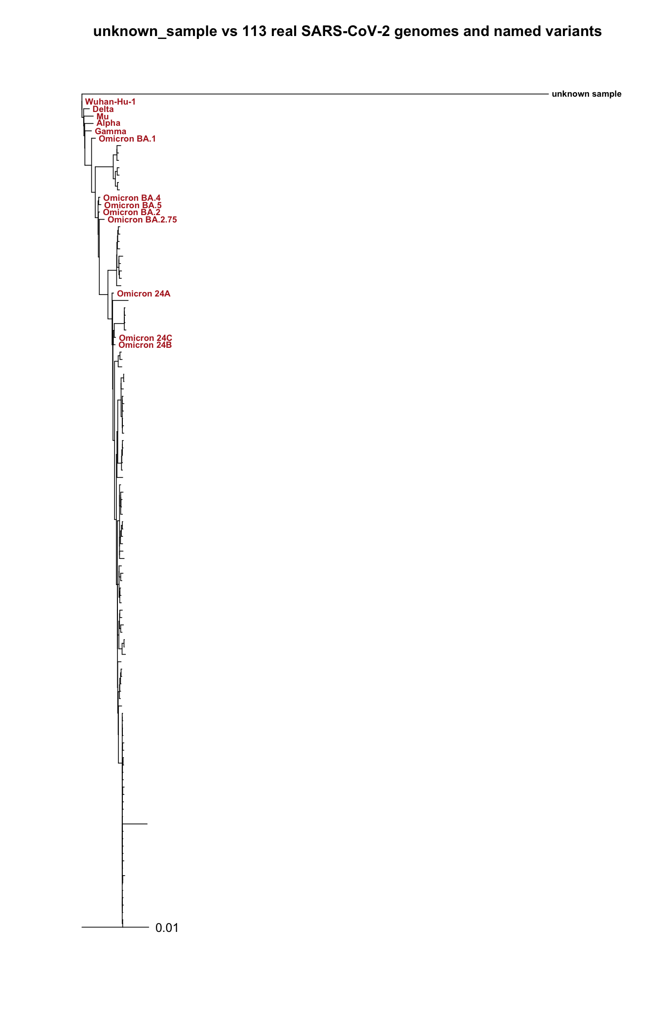
unknown_sample alone on a very long branch, the named variants near the base in the order Wuhan-Hu-1, Delta, Mu, Alpha, Gamma, then the Omicron sublineages, and the 100 background genomes (unlabelled, in grey) further down.Block D, continued (the 13 named variants only). ClipKIT trims 716 of 30,503 sites (2.35%), about twice the share trimmed from the 114-sequence alignment: with only 13 sequences, a few gappy columns weigh much more. In the EBI viewer, the Omicron columns look more similar to each other than to Wuhan_China’s, as the tree shows.
Block D2, protein vs nucleotide. SARS-CoV-2 vs SARS-CoV-1: 75.96% identity at the protein level, 74.21% at the nucleotide level. The protein is higher: several codons code for the same amino acid, so some DNA differences (synonymous substitutions) vanish at the protein level.
Section 5, your interpretation: a complete answer.
unknown_sampleis most similar to SARS-CoV-2_Wuhan-Hu-1 at every level checked: 93% nucleotide identity over nearly the whole spike gene (both BLAST searches) and the smallest whole-gene distance in the alignment table (6.9%). SARS-CoV-1 is a clear second, both by BLAST (74.2% nucleotide, 76.0% protein identity) and by distance (25.7%). MERS-CoV and HCoV-OC43 are both far more distant, around 50% whole-gene difference, and the two methods do not fully agree on which of the two is further away. This pattern suggests thatunknown_sampleshares a recent common ancestor with SARS-CoV-2, closer than its relationship to SARS-CoV-1, and is only distantly related to the other two. In the 114-genome tree, it branches apart from all real SARS-CoV-2 genomes on a much longer branch, which confirms the same conclusion by a different method.
Good limitations: the conclusion rests on a single gene; a strict BLAST search alone would have missed three of the four references; MERS-CoV and HCoV-OC43 come out in a different order depending on the method.
Optional challenge A. Rooting on a background genome does not change which variants group together, but it makes the tree start inside the SARS-CoV-2 group itself: an arbitrary choice with no biological reason. unknown_sample is a real outgroup (long branch, and different by every measure), so the root it gives shows where the group actually starts.
Optional challenge B. Distance from unknown_sample, in %:
| Reference | Raw | JC69 | Change |
|---|---|---|---|
| SARS-CoV-2_Wuhan-Hu-1 | 6.9 | 7.2 | +0.3 |
| SARS-CoV-1_Tor2 | 25.7 | 31.4 | +5.7 |
| MERS-CoV | 51.3 | 86.3 | +35.0 |
| HCoV-OC43_seasonal | 50.8 | 84.8 | +34.0 |
Saturation: over a long time, the same site can mutate several times (A to G, then back to A). The raw percentage only counts the differences still visible today, so it underestimates the real number of changes, and the more so the more distant the two sequences. A close pair has had little time for hidden changes: the correction barely moves it.
The four named reference sequences are real NCBI RefSeq records, fetched directly for this course, both as nucleotide CDS and as protein: SARS-CoV-2 (NC_045512.2, protein YP_009724390.1), SARS-CoV-1 (NC_004718.3, protein YP_009825051.1), MERS-CoV (NC_019843.3, protein YP_009047204.1), and HCoV-OC43 (NC_006213.1, protein YP_009555241.1). unknown_sample is a fifth real NCBI record, also a spike gene; its accession is kept out of this public page on purpose, since it is this session’s graded unknown. The alignment was built with MAFFT (--auto), precomputed so that the practical starts from a correct result. The SARS-CoV-2 protein accession (P0DTC2 in UniProt, YP_009724390.1 in NCBI) is the same record included in Session 1’s mystery.fasta. The bonus section’s iqtree_bonus run uses IQ-TREE’s ModelFinder and ultrafast bootstrap on this same alignment. Block D’s 114-tip tree is fetched live from NCBI by students themselves (100 arbitrary SARS-CoV-2 genomes plus 13 named variants, listed in block D, plus unknown_sample itself, added back in to check blocks B-D2’s conclusion by an independent method); sars_variants_aligned.fasta and sars_variants_tree.nwk are that same live pipeline (EntrezDirect, MAFFT --auto, FastTree -nt), run once ahead of time and kept only as a fallback. None of this is authored by this course; see NCBI, UniProt, and the ape, MAFFT, FastTree, EntrezDirect, and IQ-TREE documentation for the original data and tools.